Reader-friendly version of the 67 lecture slides: the lecture content in normal flow, with figure descriptions and data tables where the figure carries data. Open the presentation.
Slide 1
CPSY 1291Computational Methods for Mind, Brain & Behavior
Tuesday: a representation is a list of numbers, a point in a space; pixels, voxels, neurons and network units all give one; averaging over repetitions; the response matrix ; the RDM , one comparison per pair of images.
Today, part 1: what the comparison is. Euclidean distance, cosine, correlation; which of them are distances; the RDMs of pixels, people, neurons and a network.
Today, part 2: from the RDM back to a space. The psychological space: each stimulus a point, the distance between two points how dissimilar they seem to a person. Recovered from judgments alone by multidimensional scaling.
Four questions came up often enough to answer here:
"Where did the 4,096 numbers go when a row became one square of the RDM?": one number per pair, computed from both rows: the first slides today
"How different channels can provide different features": in a convolutional network, a channel is a whole sheet of units that share one set of weights, one feature detector applied at every position; the sheet shows where in the image that feature is present. Each unit is one entry of . A recording channel is one electrode, an unrelated use of the word
"Are the neural vectors per neuron, averaged over trials?": yes: one mean rate per neuron per image; Assignment 1 gives you those means
"Why 0–1 rather than 0–255?": the same 256 levels divided by 255, nothing added or lost. Networks train and run in floating point: weights and activations are real numbers, far finer than 8-bit integers, so inputs are scaled to what the weights were trained on
It is, and the pace stays: there is a lot to cover. Hardest now, at the start
The list is short: vectors, dot products, lengths, matrices, the operations every network is built from. Next week adds the eigenvector; Theme 2 the gradient
Use the help. Office hours Wednesday 1 PM, Carney 419: nobody came to talk about linear algebra
☹
Open full-size figure. TA hours are not fixed yet: vote on an Ed thread and we will set them up; I will not ask the TAs to hold hours nobody attends. Notation reference on Canvas
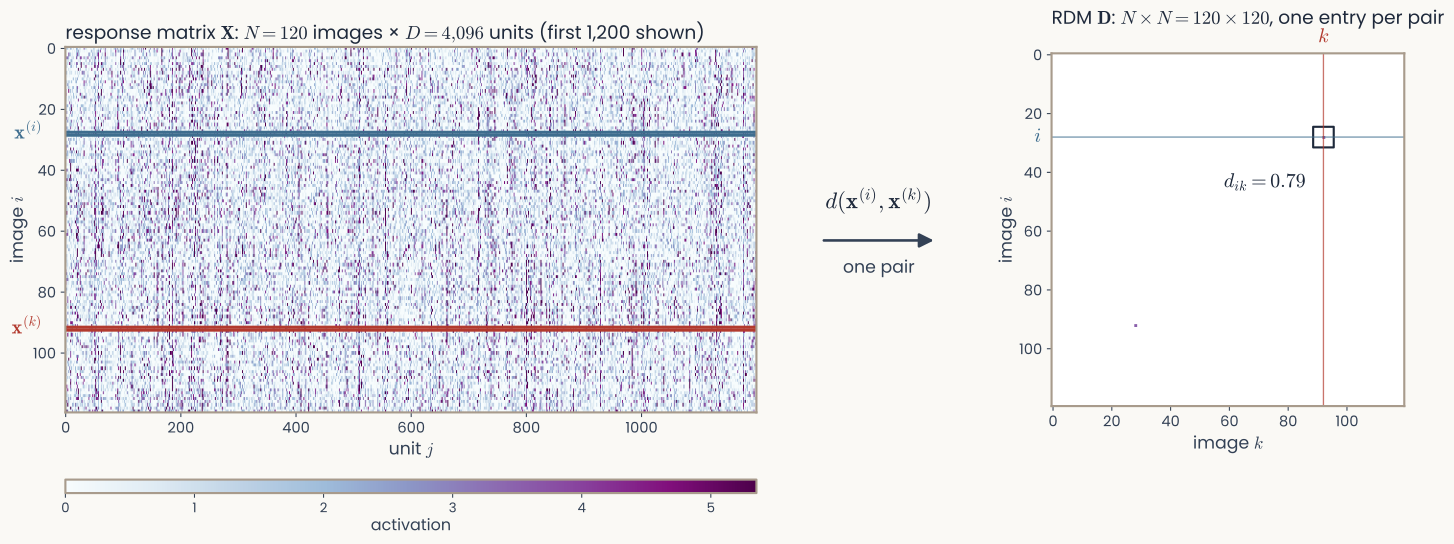
Left: the response matrix, 120 rows, one image each, 4,096 columns of unit activations, drawn as a tall strip of values with two rows highlighted; an arrow labelled with the dissimilarity measure d leads to the right: a 120 by 120 matrix with the single entry for that pair of rows highlighted
Representational dissimilarity matrix (RDM): every pairwise comparison.
Rows and columns: images, here ordered by category. Each entry: one comparison
: the dissimilarity measure. It decides which differences count
What makes it a dissimilarity matrix: zero diagonal, ;symmetric, ;nonnegative, . A fourth property, the one points in a space obey, comes later today
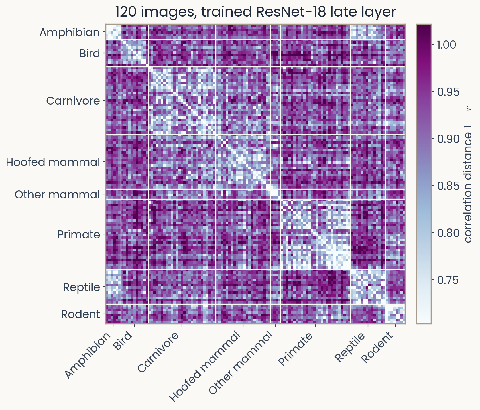
A 120 by 120 representational dissimilarity matrix of the Assignment 1 images from the trained ResNet-18 late layer, correlation distance, images ordered by animal category with category boundaries drawn; light blocks along the diagonal show that primates, carnivores and hoofed mammals are more alike within their category than across
Distance asks how far apart two points are; nothing else
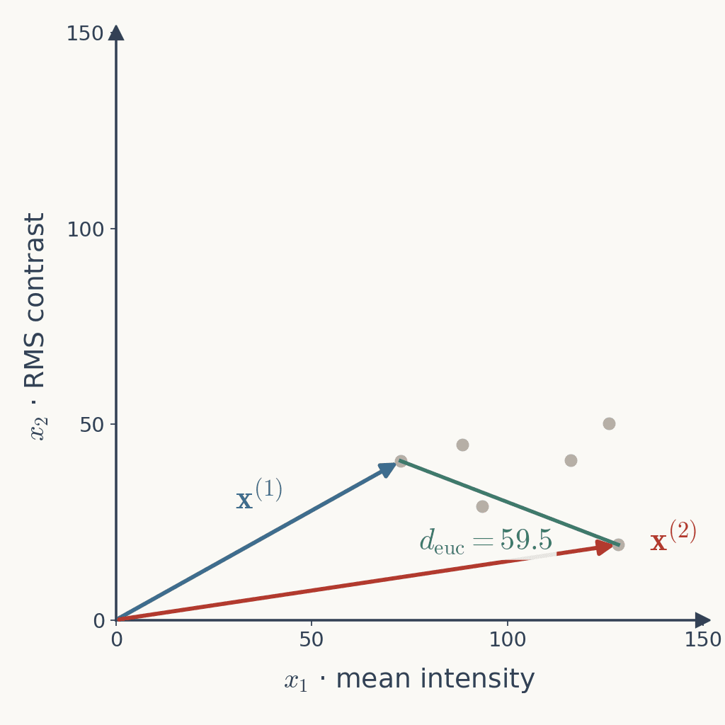
The two-feature plot, mean intensity against contrast, with the tiger's and the elephant's points; the segment between them is labelled with its Euclidean length, 59.5
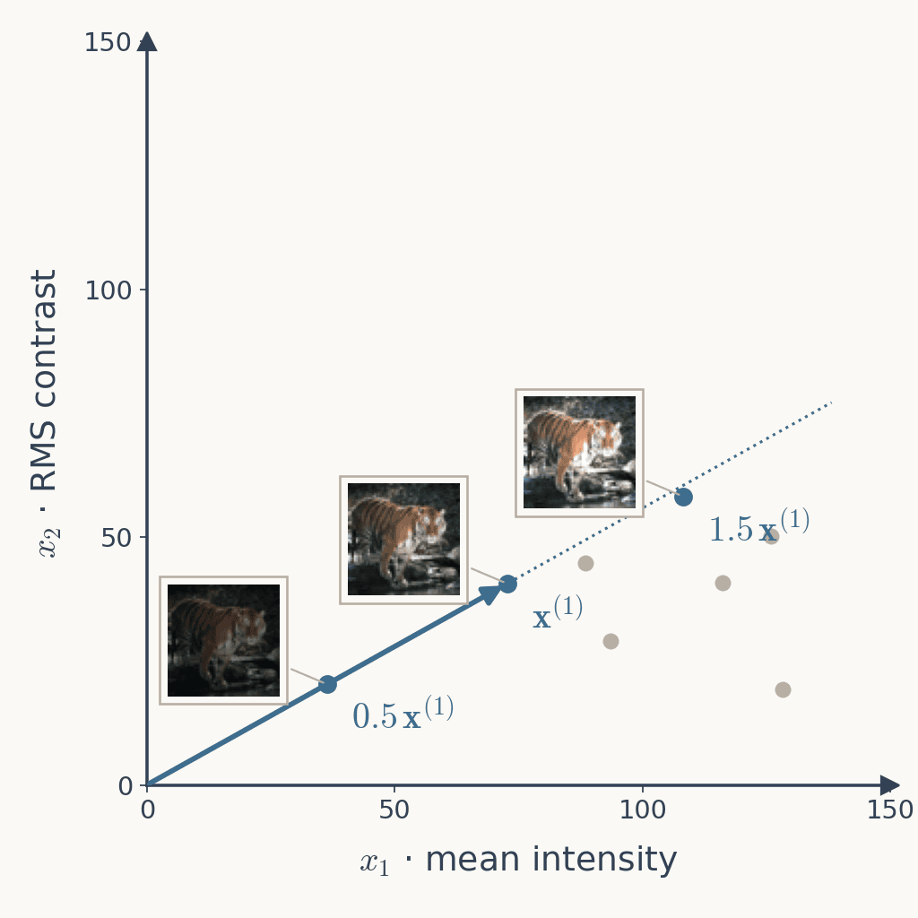
Scale every pixel by , , : the same tiger, darker or brighter. The three points lie on one line through the origin
Euclidean distance between the darkest and the brightest: , more than tiger to elephant ()
What the three share is their direction; what differs is their length. Direction = the pattern. Length = overall strength, the gain (brightness here; firing rate or activation elsewhere)
A measure of the pattern should compare directions and ignore the gain
The feature-space plot with the tiger at half, normal and one-and-a-half brightness, three thumbnails whose points lie on one dotted line through the origin, the normal tiger marked by the blue vector x superscript 1
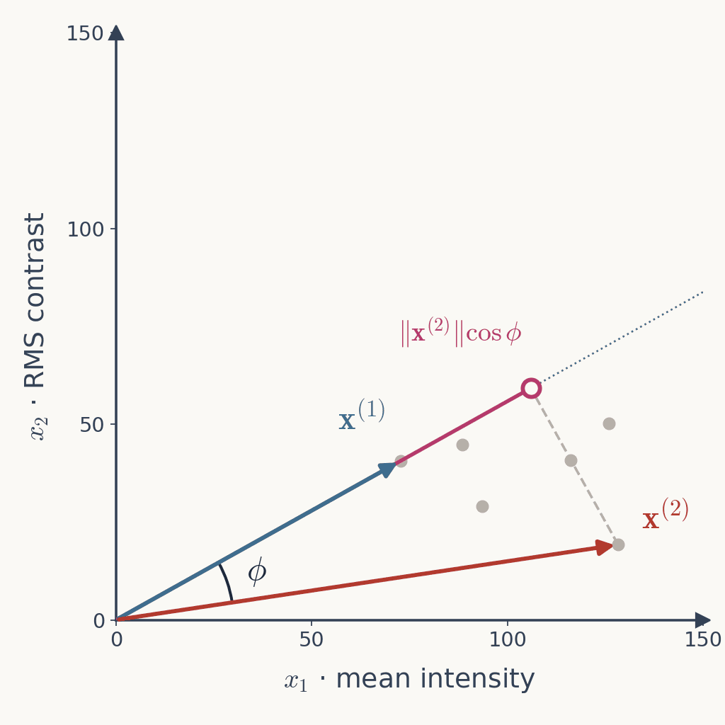
is the angle between the two vectors: when they point the same way, when perpendicular
The dot product grows with both lengths and with the alignment
Tiger and elephant: , so ,
is the projection of onto the direction of , how far reaches along it:
The feature-space plot with the tiger vector x superscript 1 and the elephant vector x superscript 2, the angle phi between them marked at the origin, and the projection of the elephant vector onto the tiger's direction shown as a magenta segment with a dashed perpendicular
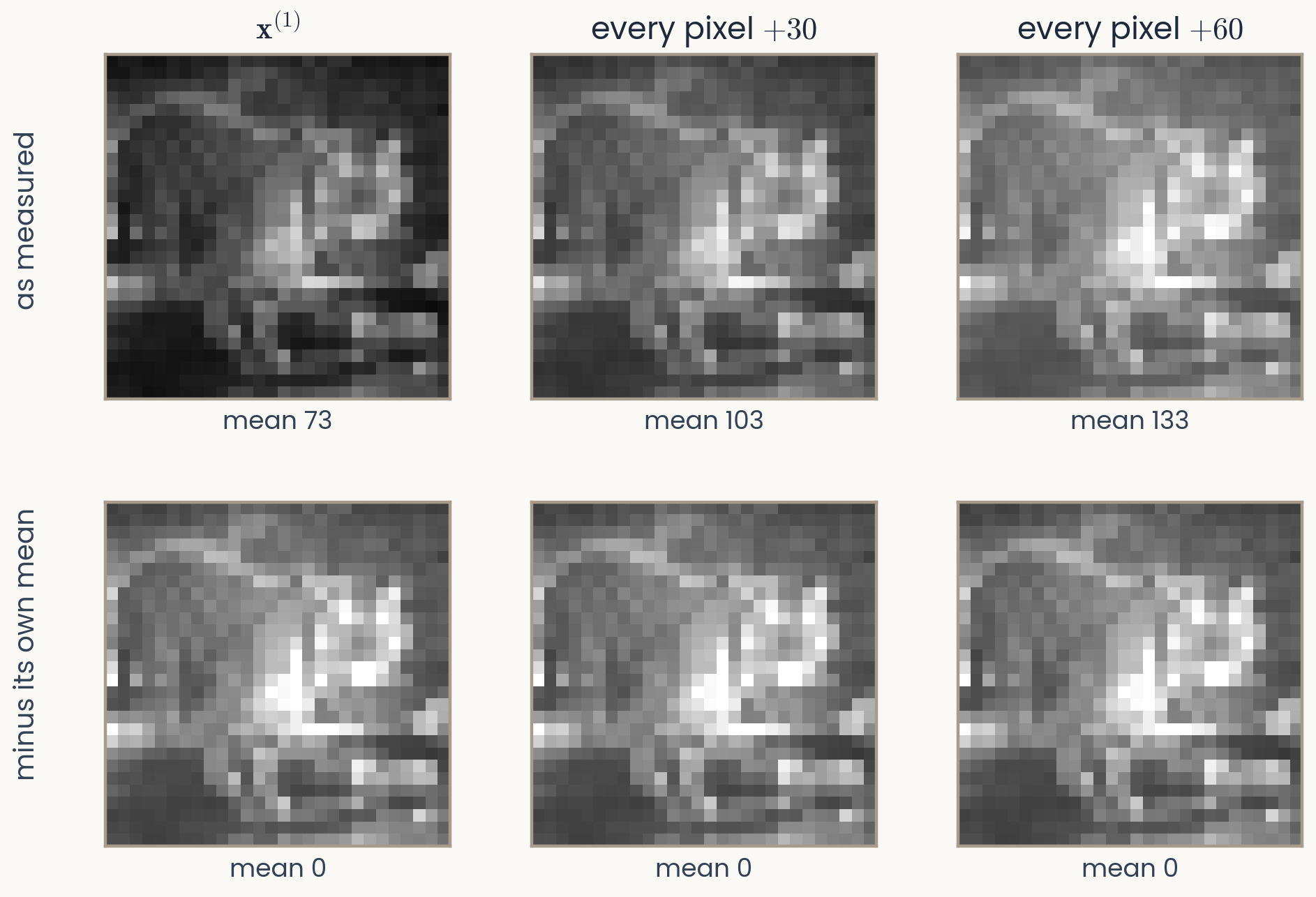
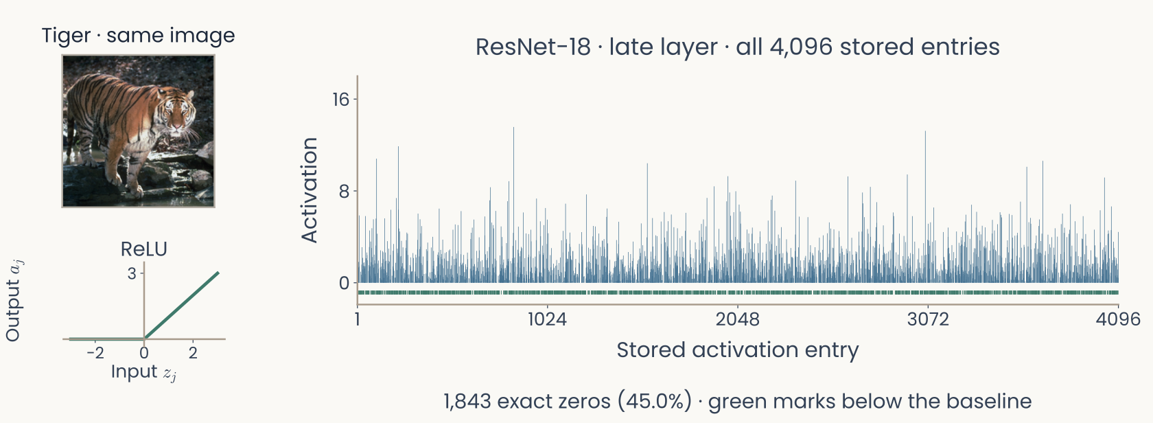
Add , then to every pixel (the 784 numbers of the 28 × 28 image): a washed-out tiger. Euclidean distance and (, : this is the 784-pixel space); , . Both report a change; the pattern did not change
Subtract each image's own mean from its pixels: the three become the same image, entry for entry
Cosine of the centred vectors is for every pair: that is correlation, next slide
A measure of the pattern should ignore a gain (last slide) and an offset (this one): a brighter image, a shift in baseline firing rate
Top row: the tiger as a 28 by 28 grey image, then with 30 and with 60 added to every pixel, progressively washed out, means 73, 103 and 133. Bottom row: each image minus its own mean, three identical images with mean 0
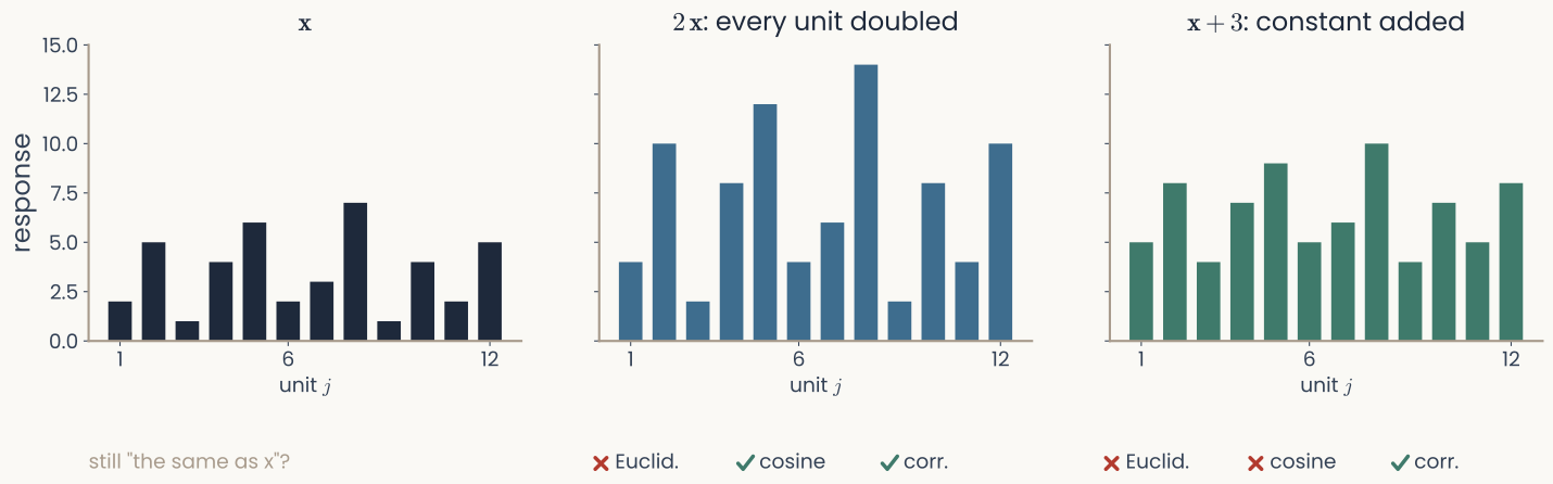
Three bar charts of a twelve-unit response pattern: the pattern itself, every unit doubled, and a constant added to every unit; under each, marks show which measures call it the same as the original: Euclidean distance none, cosine similarity only the doubled pattern, correlation both
Which is closer to the tiger? It depends on the measure
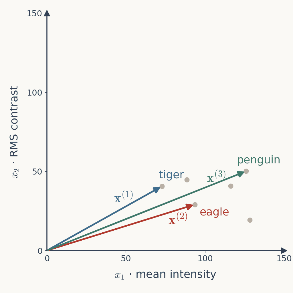
Two features (plot): eagle or penguin?
Which is closer to the tiger? It depends on the measure — table
Pair
Euclidean
Cosine*
Correlation*
tiger–eagle
23.8
0.021
0†
tiger–penguin
54.1
0.009
0†
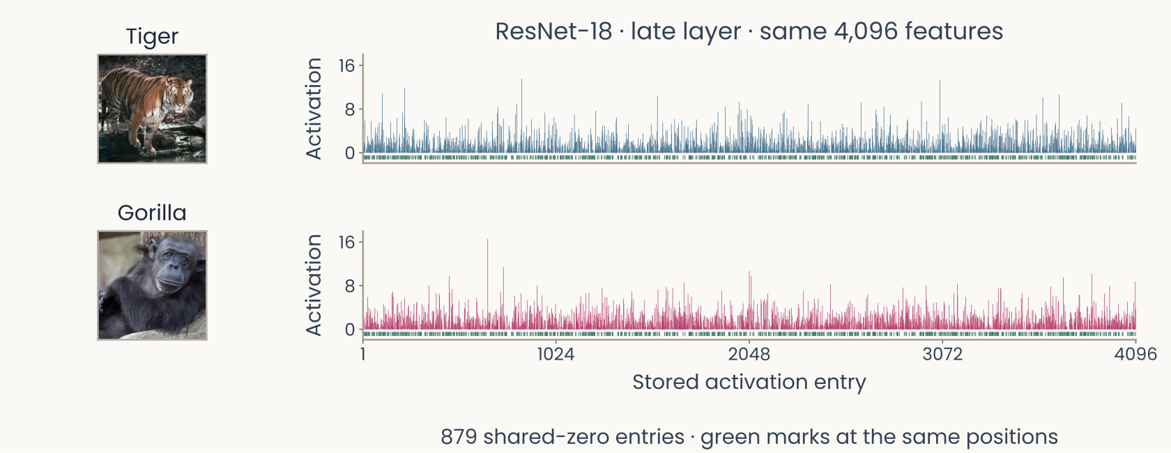
4,096 network responses: penguin or gorilla?
Which is closer to the tiger? It depends on the measure — table
Pair
Euclidean
Cosine*
Correlation*
tiger–penguin
122.8
0.649
0.911
tiger–gorilla
125.7
0.635
0.897
* dissimilarities, and · † with two components, always: correlation needs more than two
The two-feature plot with three arrows from the origin: the tiger x superscript 1, the eagle x superscript 2, and the penguin x superscript 3. The eagle's point is nearer the tiger's, but the penguin's arrow is more nearly parallel to the tiger's
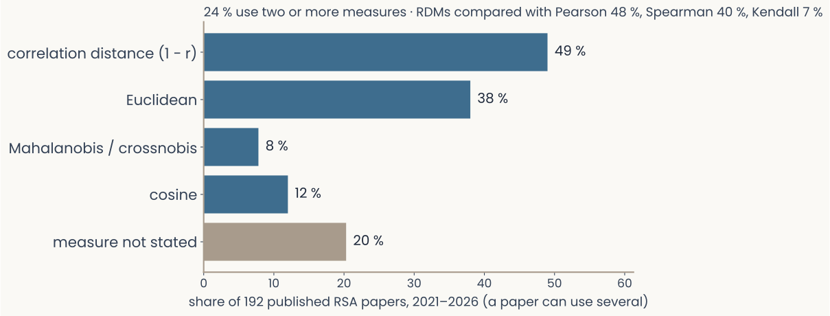
Horizontal bar chart over 192 published RSA papers from 2021 to 2026: correlation distance 49 percent, Euclidean 38, Mahalanobis or crossnobis 8, cosine 12, measure not stated 20 percent; the title says 24 percent use two or more measures and that RDMs are compared with Pearson in 48 percent, Spearman in 40, Kendall in 7
Correlation distance first, Euclidean next, cosine and a few others behind. The field uses them interchangeably, and one paper in five never says which one it used
They are not interchangeable: the last slides showed each one ignoring something different. That is why you build all three in Assignment 1 and say which you used, and why
RDMs are compared with two different correlations about equally often; the assignment uses the rank-based one, the end of today
192 open-access papers that compute an RDM, 2021–2026, Europe PMC full text; the measure counted automatically · an estimate
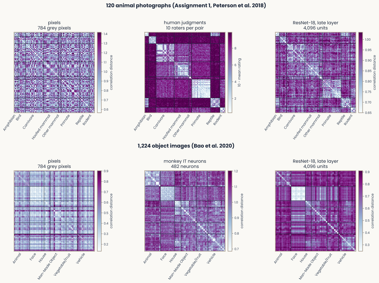
Six dissimilarity matrices in two rows, images ordered by category with boundaries drawn, each on its own colour scale. Top row, the 120 animal photographs: pixels show no block structure, human judgments show strong light blocks on the diagonal, one per category, the ResNet-18 late layer shows partial blocks. Bottom row, the 1,224 object images of Bao and colleagues: pixels show faint structure, monkey IT neurons show clear blocks for faces and animals, the ResNet-18 late layer shows a strong face block
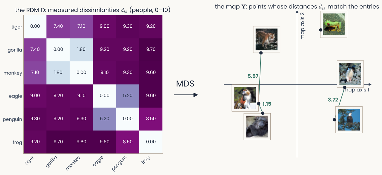
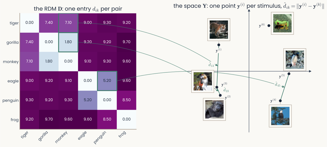
Left: the 6 by 6 human dissimilarity matrix of a tiger, a gorilla, a monkey, an eagle, a penguin and a frog, entries printed. Right: the two-dimensional map that MDS returns, a dot per animal with its thumbnail beside it, three map distances written on their segments: tiger to monkey 5.57, gorilla to monkey 1.15, eagle to penguin 3.72
So far: responses in, a matrix out. Now the reverse: a matrix in, points out. Six animals rated by people (: 0 identical, 10 nothing in common) to six points on a plane whose distances come as close as possible
Gorilla–monkey rated , on the map; eagle–penguin , . No plane reproduces all fifteen numbers at once; how close one can get is measured later today
A long tradition in psychology: what we know of objects is arranged as points in a space, near when alike. That psychological space cannot be measured directly. What can be measured is a judgment. Peterson and colleagues asked people: how similar are these two images, from 0 to 10? Ten raters for every pair of 120 animal photographs.
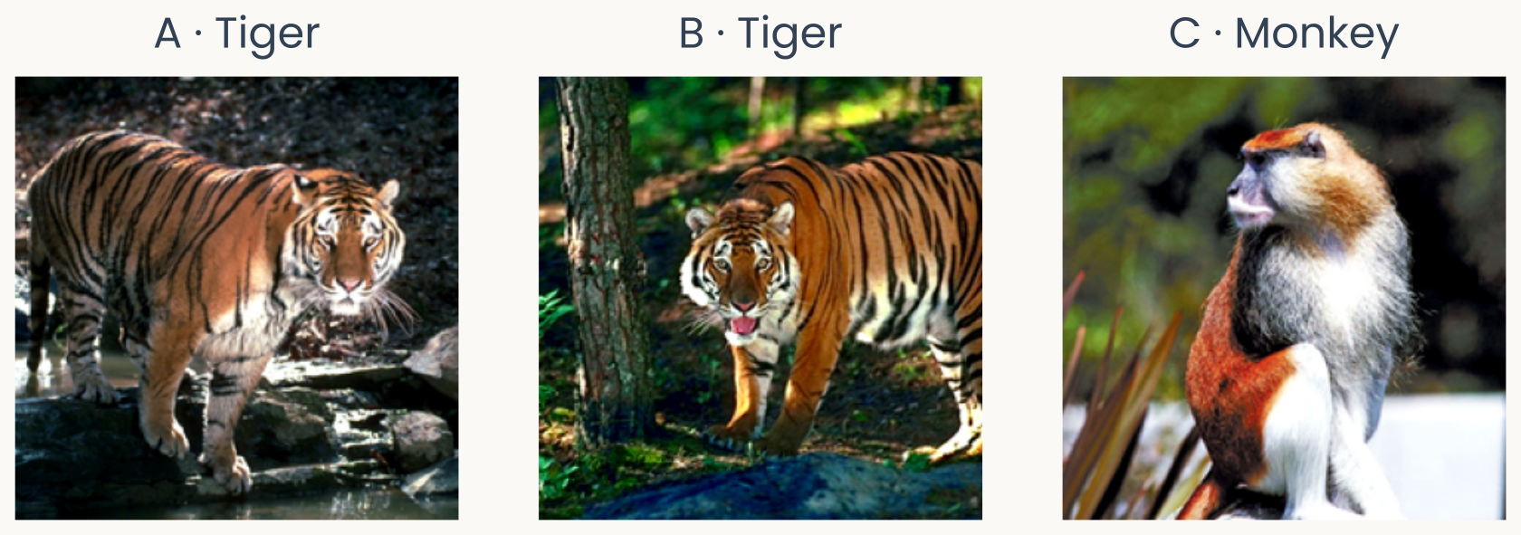
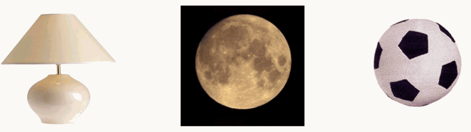
Two tiger photographs A and B and a monkey photograph C, from the Assignment 1 image set
Will it work? Yes, if the matrix is, or is well approximated by, a table of distances between points in that space. What a table of distances must satisfy, and which of our measures satisfy it:
Which measures are distances in the full sense? — table
Requirement
Mathematical statement
Euclidean
Cosine
Correlation
Nonnegativity · no negative distances
✓ Yes
✓ Yes
✓ Yes
Identity · zero only for an image and itself
✓ Yes
✗ No
✗ No
Symmetry · same both ways
✓ Yes
✓ Yes
✓ Yes
Triangle · no shortcut via a third image
✓ Yes
✗ No
✗ No
A distance in the full sense (a metric)?
All four
✓ Yes
✗ No
✗ No
✓ holds throughout the domain; ✗ can fail even when the measure is defined. On our images: 2.3 % of pixel triples break the triangle inequality under cosine, none in the trained late layer, and a brighter copy of an image sits at cosine distance 0 from it. You test this yourself: Assignment 1 bonus B1 · worked examples in the appendix.
The six-animal dissimilarity matrix on the left with three entries outlined, tiger–monkey, gorilla–monkey and eagle–penguin, each joined by an arrow to the segment between the corresponding two points on the map on the right, where every point is labelled y with its stimulus number and each segment is labelled d-hat with the pair's indices
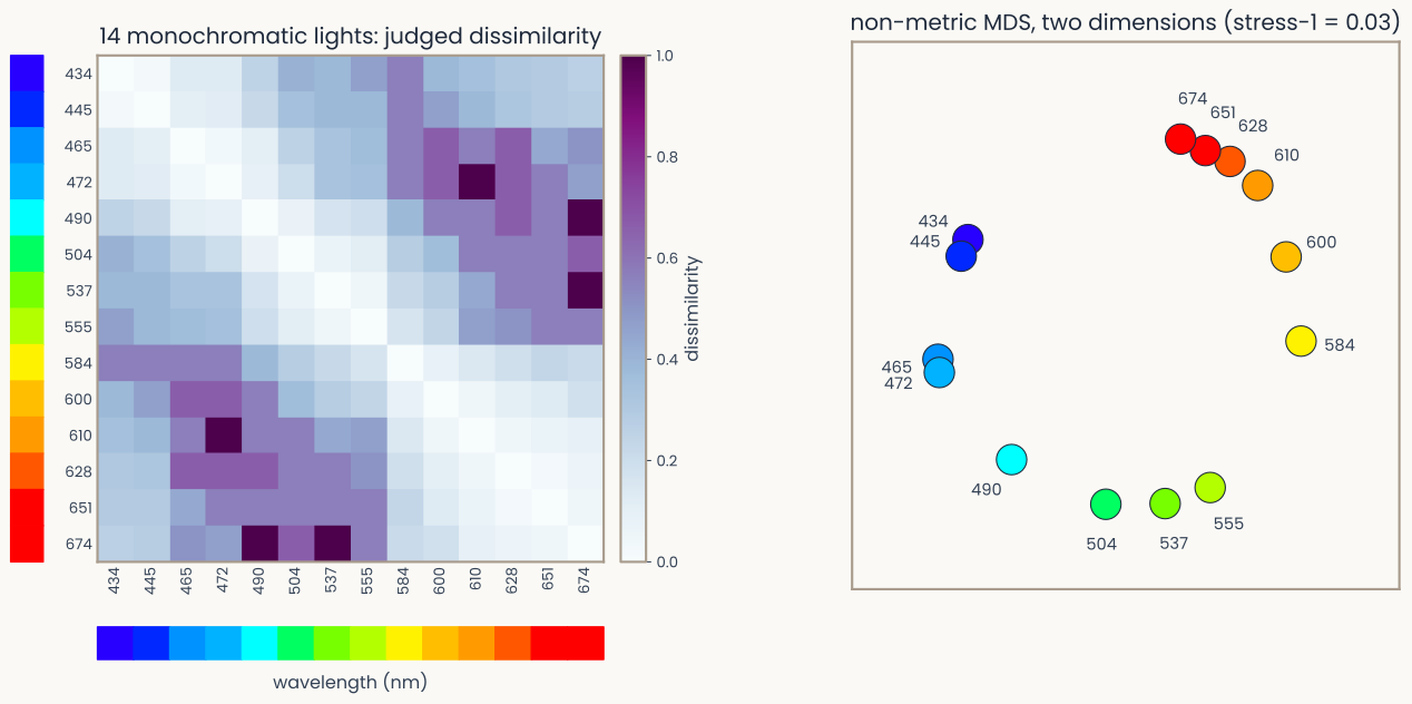
Left: Ekman's 14 by 14 matrix of judged dissimilarity between monochromatic lights from 434 to 674 nanometres, with a wavelength colour strip along each edge. Right: the two-dimensional non-metric MDS solution, each light drawn in its own colour: a circle, violet next to red
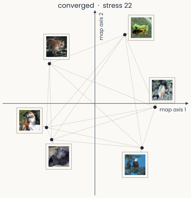
The six animals at convergence, the map MDS returns for the six-animal ratings: gorilla and monkey close together, eagle and penguin close together; stress 22
The mismatch, as a fraction of the map's own spread. : every distance matches. : mismatches about a third the size of the distances
Raw stress depends on the units of ; Stress-1 does not, so fits can be compared across data sets and dimensions
sklearn can print it. Rule of thumb (Kruskal 1964): 0.05 excellent · 0.10 fair · 0.20 poor. Assignment 1 §2e adds a real check: the stress of the same fit on a shuffled matrix, which has no structure to recover
The assignment gives you the call and takes you through it one step at a time
The solution is not unique. Shift, rotate or reflect the configuration: pairwise distances unchanged, stress unchanged. The axes mean nothing. Only relative positions do
The dimension is your choice. Plot stress against : it always falls; look for the elbow. Two dimensions is a display convenience
Low stress ≠ true. Enough dimensions fit anything, noise included. Report normalized stress (Stress-1) and the number of dimensions
If a story about your map depends on which way is "up", it is a story about the plot.
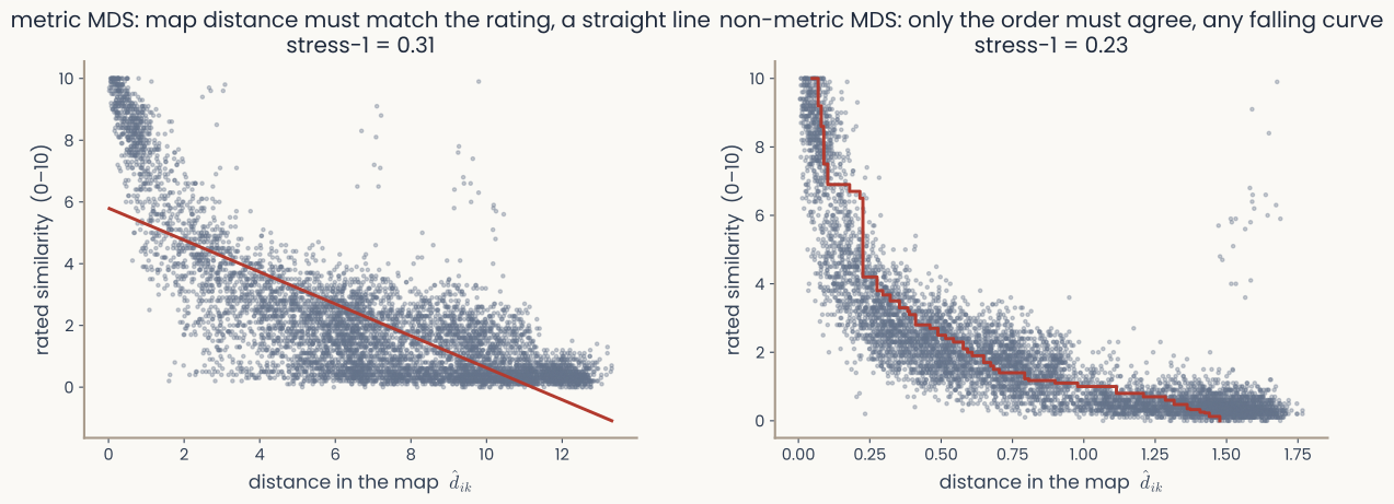
Two scatter plots of rated similarity, 0 to 10, against distance in the recovered map for the 120 animal ratings. Left, metric MDS: the fitted relation is a straight falling line, stress-1 0.31. Right, non-metric MDS: the fitted relation is a falling step curve, stress-1 0.23; the points bend because ratings pile up near 0
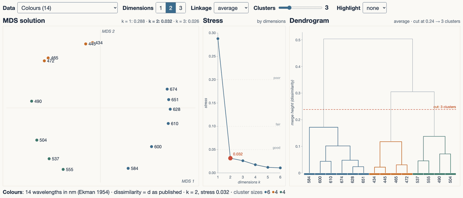
Left: nonmetric MDS map of Ekman's 14 colours, a circle ordered by wavelength. Middle: stress against the number of dimensions, falling from 0.29 in one to 0.03 in two. Right: the dendrogram of the same dissimilarities cut at three clusters
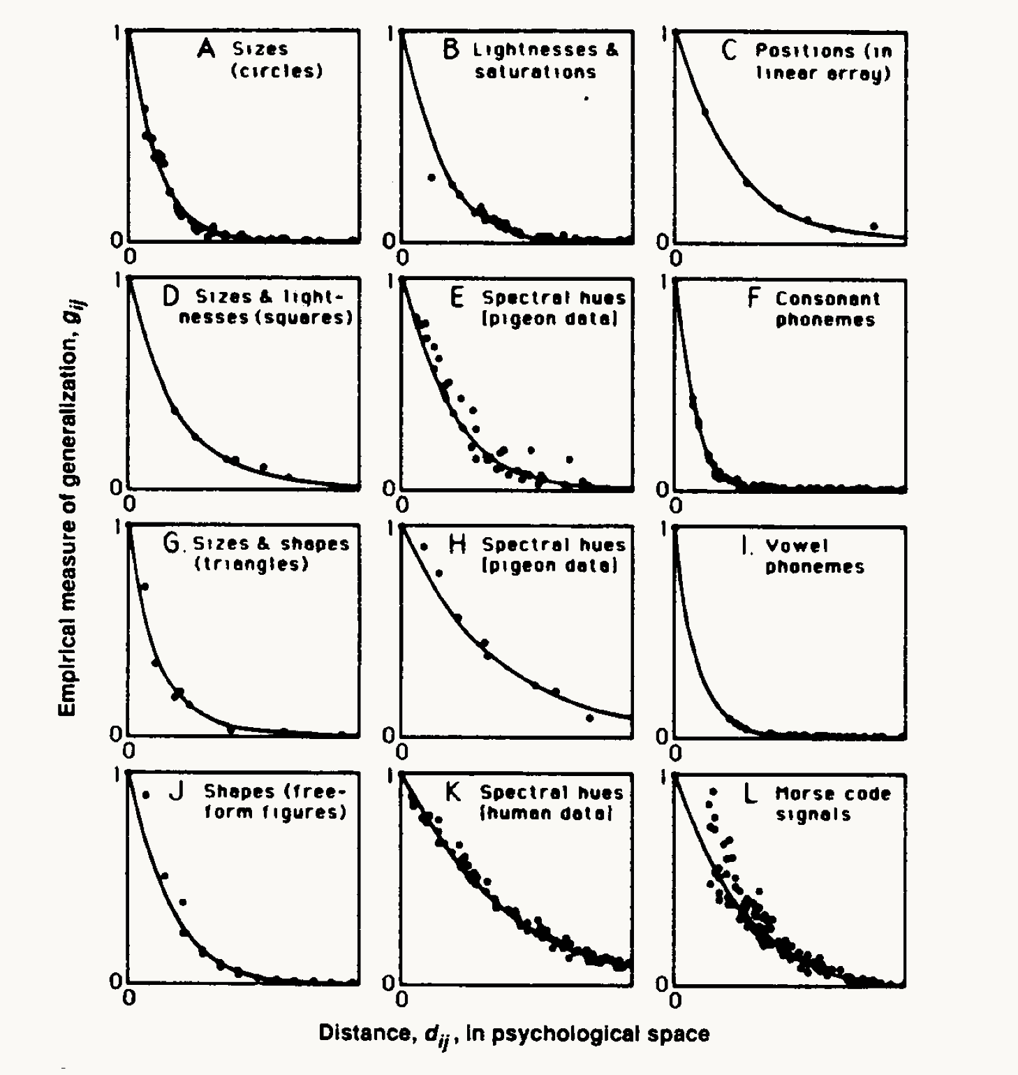
Twelve small panels of generalization plotted against distance in psychological space — sizes, hues, phonemes, Morse code, human and pigeon data — each tracing the same exponential decay
Recover the psychological space by non-metric MDS (Shepard 1962, Kruskal 1964) from confusions or ratings; then plot measured generalization against distance in that space. Twelve datasets, one curve:
Similarity is an exponential function of psychological distance, and the law is not circular: non-metric MDS fits rank order only, so the exponential shape was never built in.
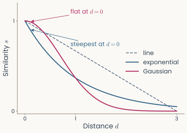
Assignment 1 §2g fits three curves to the same (distance, similarity) pairs:
The line is the baseline: constant-rate decay, no law to state
Any bend beats a line, so the fair rival is the Gaussian: same two parameters, but flat at where the exponential is steepest
The test is at the origin: which shape do the pairs follow there?
Preview: in the space recovered from people the exponential wins; against a network's distances the picture changes, because a network's distance is a different ruler from psychological distance
Exponential and Gaussian similarity curves with the same value at zero but different initial slopes
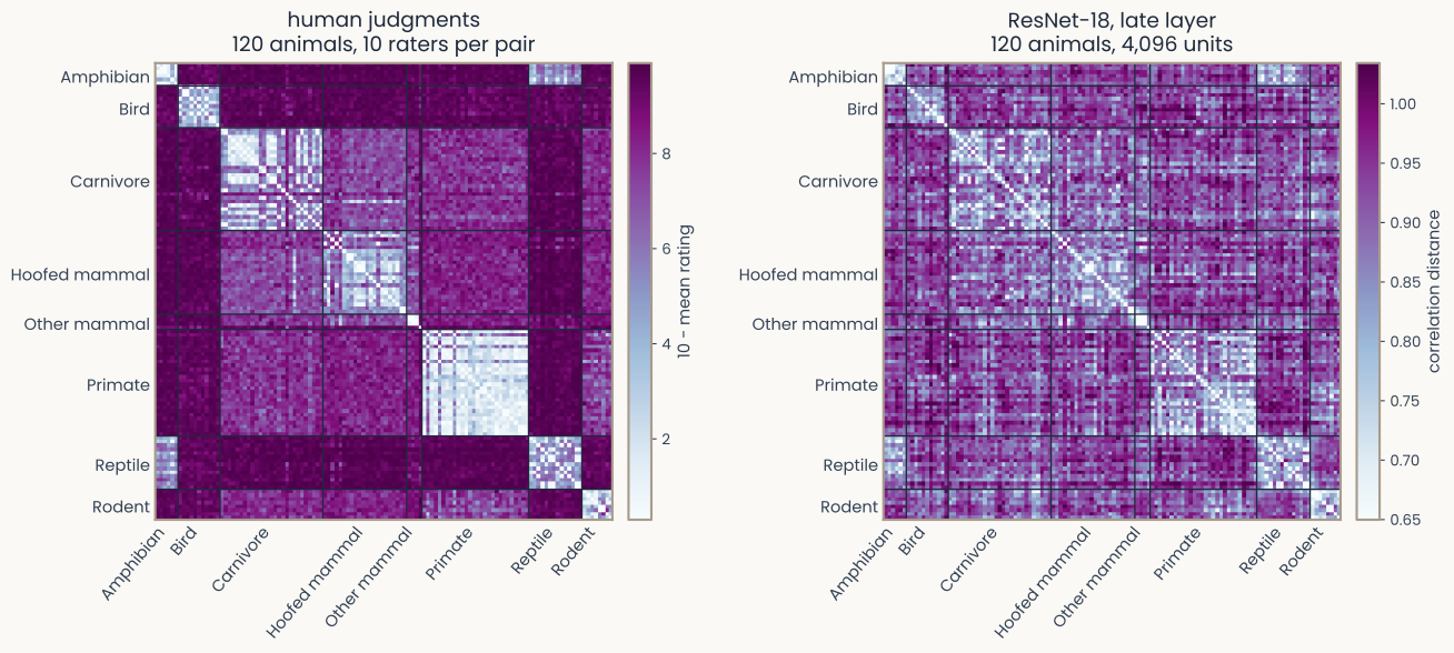
Two 120 by 120 dissimilarity matrices of the same animals, ordered by category with category boundaries drawn: human judgments on the left with strong light blocks along the diagonal, the ResNet-18 late layer on the right with weaker blocks in the same places
Two 120 by 120 dissimilarity matrices of the same animals side by side, human judgments and the ResNet-18 late layer, both with light blocks along the diagonal, weaker for the network
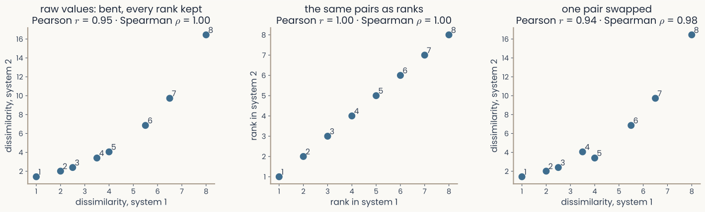
Three scatter plots of eight pairs' dissimilarities in two systems. Left: the second system's values are a bent but rising function of the first's, Pearson 0.95, Spearman 1. Middle: the same eight pairs plotted as ranks, a perfect straight line. Right: two neighbouring pairs swapped, Pearson 0.94, Spearman 0.98
Two systems, the same stimuli, two matrices: from the judgments, from a layer. Flatten each upper triangle into a list of numbers and correlate the two lists:
In practice: iu = np.triu_indices(N, k=1), then spearmanr(D1[iu], D2[iu]).
The operation has a name: representational similarity analysis, RSA
Upper triangle only. The diagonal is zeros in both matrices, agreement you did not measure; the lower half copies the upper. Either one inflates agreement or the sample size
Rank correlation (Spearman): the two systems share no scale, a distance between voxel patterns and one between unit activations being different kinds of number. The raw values are not comparable; their order is
The two matrices of a moment ago: . Pearson on the same lists gives , a different question
The two systems order the pairs alike: what one treats as close, the other tends to treat as close. A claim about geometry, and only that
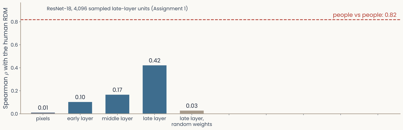
alone means little. It needs how well people agree with each other (the noise ceiling, two slides on) and a second model: something to be large relative to
Assignment 1 reports Spearman between the human matrix and ResNet-18's correlation distances: expect about 0.4. Whether that is good: two slides on
Matching geometry is evidence about a representation, not a demonstration of shared mechanism.
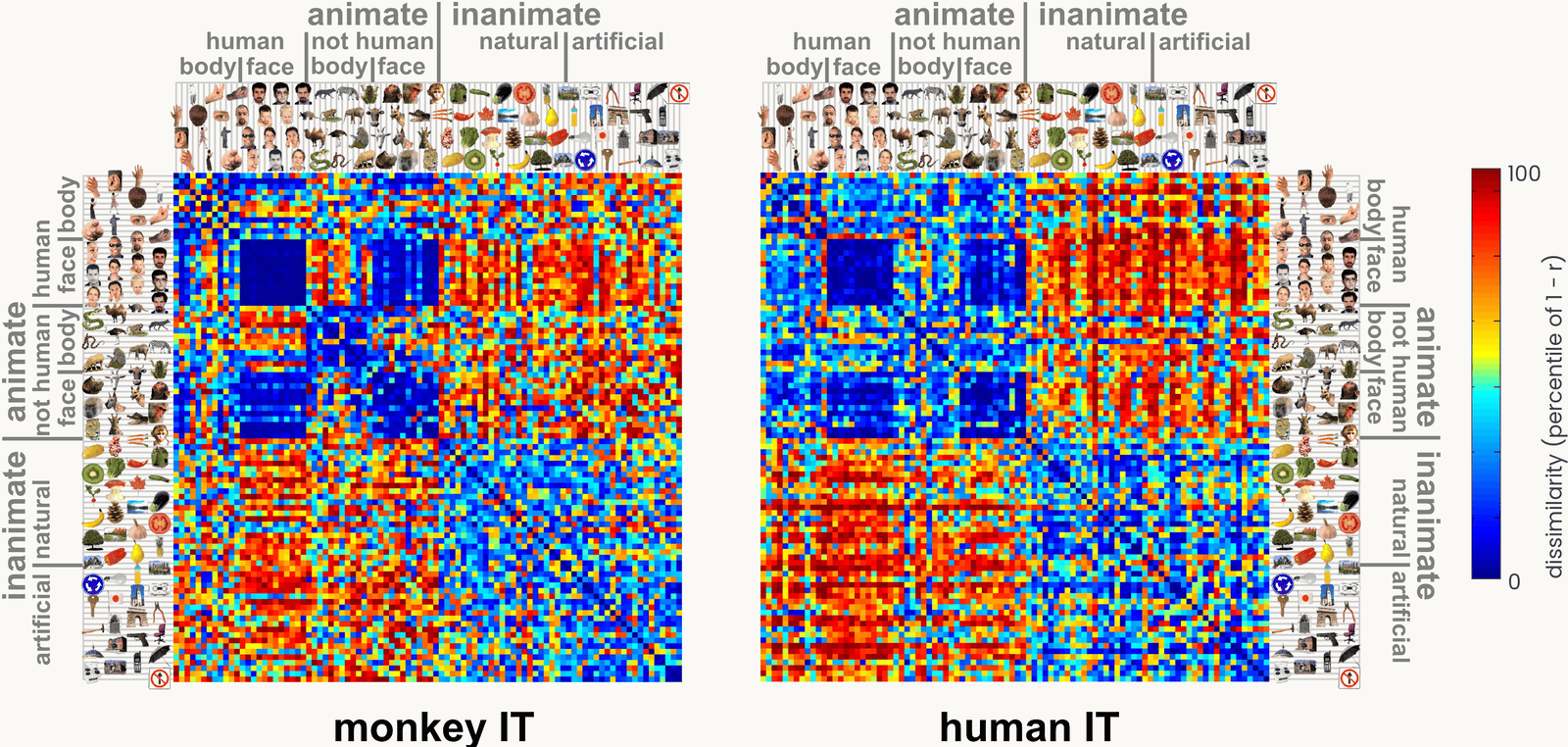
Two 92-by-92 dissimilarity matrices, monkey IT from single-unit recordings and human IT from fMRI, both showing the same blue animate block and warm inanimate block with face and body sub-blocks; a vertical colour bar on the right runs from blue, similar, to red, dissimilar
Bar chart of Spearman correlation between the human RDM and five candidate RDMs on the 120 animal images: pixels 0.01, early layer 0.10, middle layer 0.17, late layer 0.42, late layer with random weights 0.03; a dashed line at 0.82 marks the agreement between two independent groups of raters
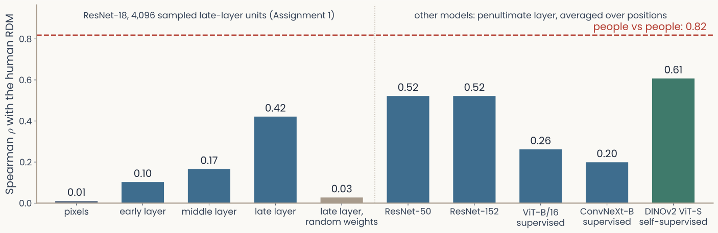
Bar chart of Spearman correlation with the human RDM for five models using pooled penultimate features: ResNet-50 0.52, ResNet-152 0.52, supervised ViT-B/16 0.26, ConvNeXt-B 0.20, self-supervised DINOv2 ViT-S 0.61 in green; dashed ceiling at 0.82
It is long. Start now if you have not; it is due Tuesday, September 29
After today you have everything for Parts 1 and 2 (distances, RDMs, MDS, Shepard's law, the RDM comparison). Part 3 is Tuesday's lecture (PCA); the bonus has no lecture of its own
The assignment is written to be self-sufficient: every part explains what it needs. Starting a part before its lecture is allowed and often useful; the lecture then lands on something you have already tried
Bonus B2 (hierarchical clustering) is not taught in class: the clustering slides in the appendix are what you need
A dissimilarity matrix turns any responses (neurons, voxels, model units, judgments) into one object, whatever the measurement system
MDS turns that matrix into a map by lowering the stress. Axes mean nothing; relative positions do
Shepard's law: similarity falls off exponentially with distance in psychological space
People's judgments need not obey the triangle inequality (appendix). Treat the map as a useful approximation
The same matrix can be read as a tree of nested categories instead of a flat space (clustering, in the appendix)
Representational similarity analysis: correlate the upper triangles of two such matrices; one number for how far two systems agree about what resembles what
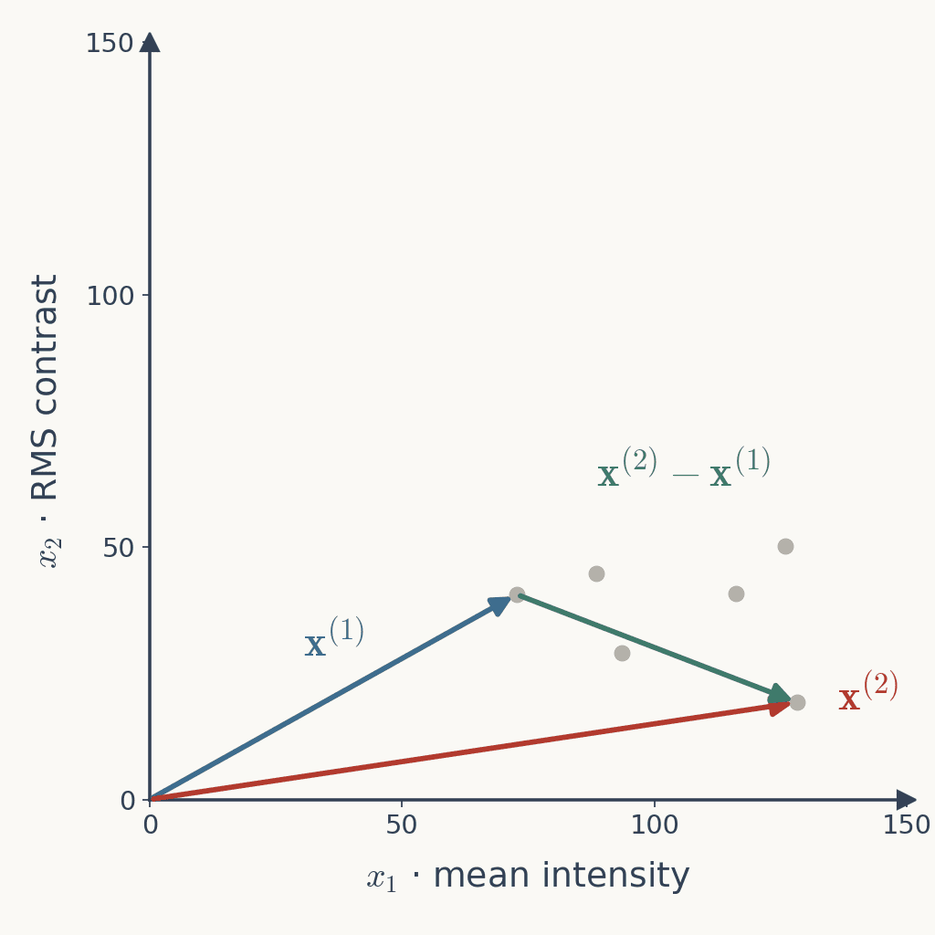
Subtraction: the displacement from image 1 (tiger) to image 2 (elephant):
is itself a vector: from the tiger's point to the elephant's.
The two-feature plot, mean intensity against contrast, with three arrows: x superscript 1 to the tiger's point, x superscript 2 to the elephant's point, and their difference drawn from the tiger's point to the elephant's
Appendix · Computing an RDM from a response matrix
import numpy as np
from scipy.spatial.distance import pdist, squareform
R = np.load("responses.npy") # (N stimuli, n channels)print(R.shape) # (120, 4096) units or (120, 482) neurons# pdist returns the upper triangle: N(N-1)/2 numbers, the pairs i < k
d_vec = pdist(R, metric="correlation") # 1 - Pearson r, pattern to pattern
D = squareform(d_vec) # (N, N): symmetric, zero diagonalassert np.allclose(D, D.T) and np.allclose(np.diag(D), 0)
pdist computes only the upper triangle, never the matrix. squareform converts either way
Swap metric="euclidean" (or "cosine") to change the geometry; nothing downstream changes
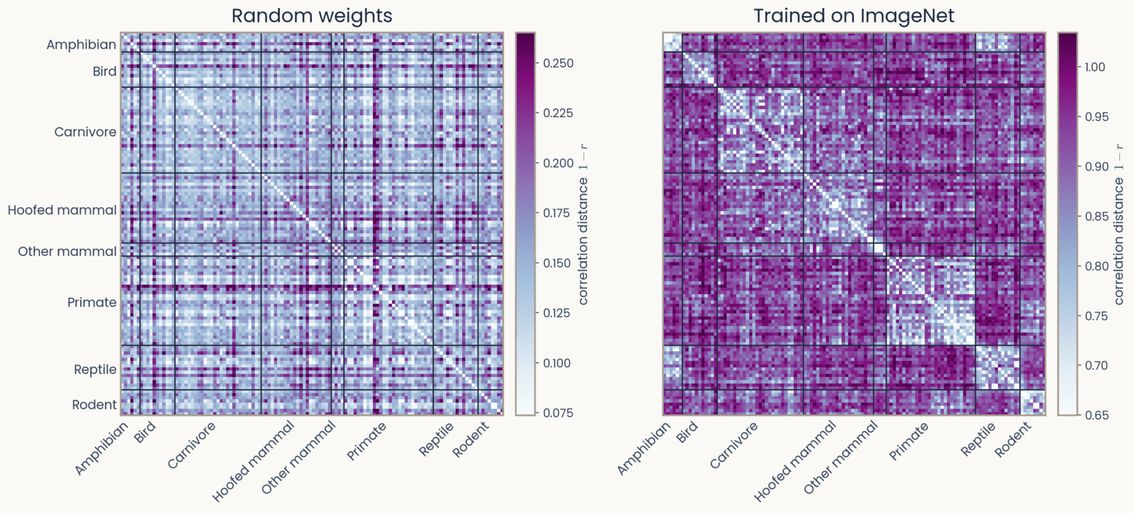
Two 120-by-120 correlation-distance RDMs of the late ResNet-18 layer, images ordered by category with dark lines at the category boundaries, each on its own colour scale: with random weights the entries are noise with no block structure; with ImageNet-trained weights lighter blocks sit on the diagonal, one per category
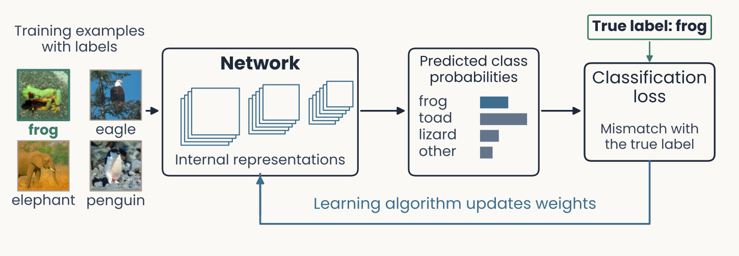
Weights: the adjustable numbers inside the network. Training: find weights that reduce the classification loss on labeled images
Supervised training: four labelled training photographs (frog, eagle, elephant, penguin) pass one at a time through a network to produce class predictions; comparing the prediction with the true label gives a loss, which guides weight updates and changes internal representations
Similarity ratings come from people, not from a formula. A network's RDM inherits its properties from the measure ; a rater is free to answer anything. Before we recover a space from such numbers, what must they satisfy? For tiger, penguin, gorilla ():
The tiger against itself: no difference. (zero diagonal)
Tiger against penguin, penguin against tiger: the same number. (symmetric). A rater need not agree (Tversky 1977: a camel is judged more like a horse than a horse like a camel)
No difference below zero. (nonnegative)
Tiger to gorilla is never more than tiger to penguin plus penguin to gorilla: (triangle inequality). Nothing stops a rater from breaking it
The first three make a dissimilarity matrix. The fourth is what points in a space obey: without it, no map reproduces the entries exactly. Which measures satisfy which: the distance table in the lecture. Whether people do: the assignment bonus, and the Tversky slides later in this appendix
from sklearn.manifold import MDS
mds = MDS(n_components=2, # m = 2, because we want to look at it
metric="precomputed", # feed D directly, NOT the raw R
n_init=8, normalized_stress="auto", random_state=0)
Y = mds.fit_transform(D) # (N, 2) coordinates - one row per stimulusprint(Y.shape, mds.stress_) # residual mismatch: lower is better# non-metric (ordinal) MDS - fits the RANK ORDER of the dissimilarities
mds_nm = MDS(n_components=2, metric="precomputed", metric_mds=False,
n_init=8, normalized_stress="auto", random_state=0)
Y_nm = mds_nm.fit_transform(D)
metric="precomputed" (dissimilarity= before scikit-learn 1.8); without it sklearn treats D as raw data and computes Euclidean distances from it
D must be the square matrix: squareform(d_vec) first if you kept the pdist vector
n_init=8: stress-based MDS has local minima, so restart and keep the best
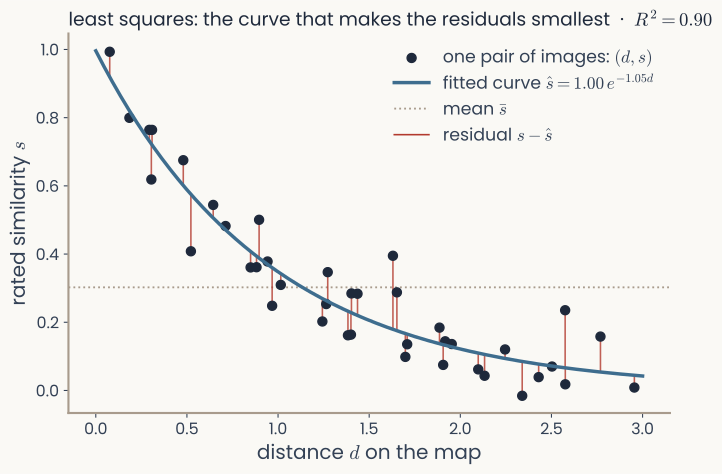
Each point is one pair of images: its map distance and its rated similarity
Fit = choose the curve's parameters (, ) so the curve passes as close as possible to the points: smallest sum of squared residuals . Same idea as fitting a line, the curve just bends
= the share of the spread in the curve accounts for: perfect, no better than the flat mean
Fit the three curves to the same points, compare their ; the highest wins, the line is the baseline
Scatter of forty distance–similarity pairs with a fitted exponential curve through them, a vertical residual segment from every point to the curve, a dotted horizontal line at the mean similarity, and R squared 0.90 in the title
Appendix · Human reliability sets the comparison scale
Split-half reliability: correlate two independent sets of ratings for the same pairs. That agreement is the noise ceiling: how well the measurement predicts itself, the bar no model should beat.
Appendix · Human reliability sets the comparison scale — table
Comparison
Statistic
Rating half 1 versus rating half 2
Reliability of the human measurement
Network distances versus human dissimilarities
Representational alignment
Assignment 1 uses Spearman rank correlation for both quantities. Pearson , Spearman and regression are different statistics
Peterson's two rater batches agree at Spearman on our 120 images. Report a model as a fraction of the ceiling: late layer / ceiling
The averaged ratings are more reliable than either half, so that fraction is an upper bound on what the model has reached
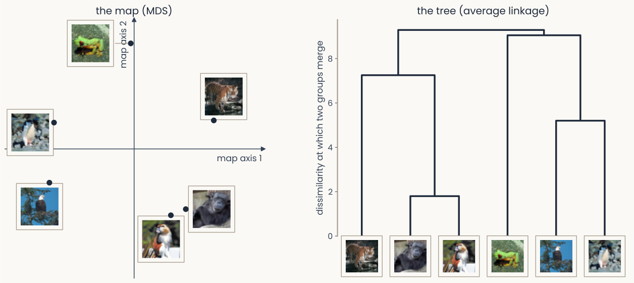
Left: the two-dimensional MDS map of six animals, tiger, gorilla, monkey, eagle, penguin, frog, thumbnails beside the points. Right: the dendrogram built from the same six-by-six human dissimilarity matrix with average linkage, thumbnails as leaves; gorilla and monkey join at 1.8, eagle and penguin at 5.2, the frog joins last
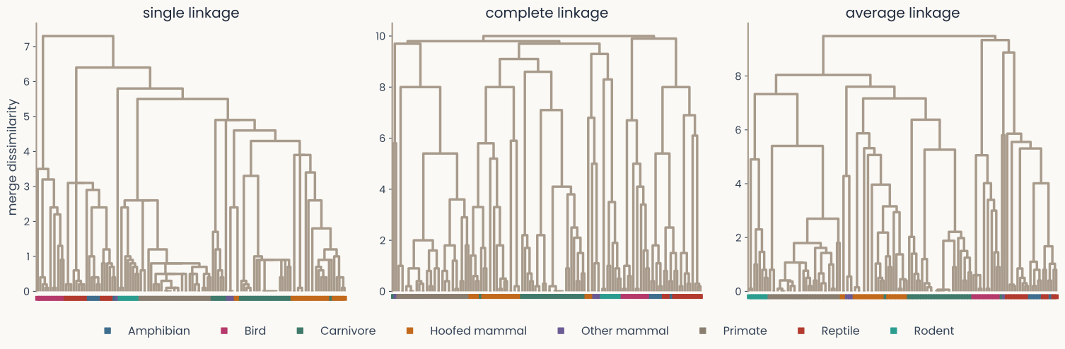
Three dendrograms of the same 120 animals from the human dissimilarity matrix, single, complete and average linkage, each leaf marked with its taxon colour: single linkage grows one long chain, complete linkage makes compact groups, average linkage sits between
Same 120 animals, same human ratings, three linkage rules: three different trees. The colours under the leaves are the eight taxa
Single linkage chains: one long thin cluster forms by hopping neighbor to neighbor. Complete linkage forces compact groups, which can split an elongated one.
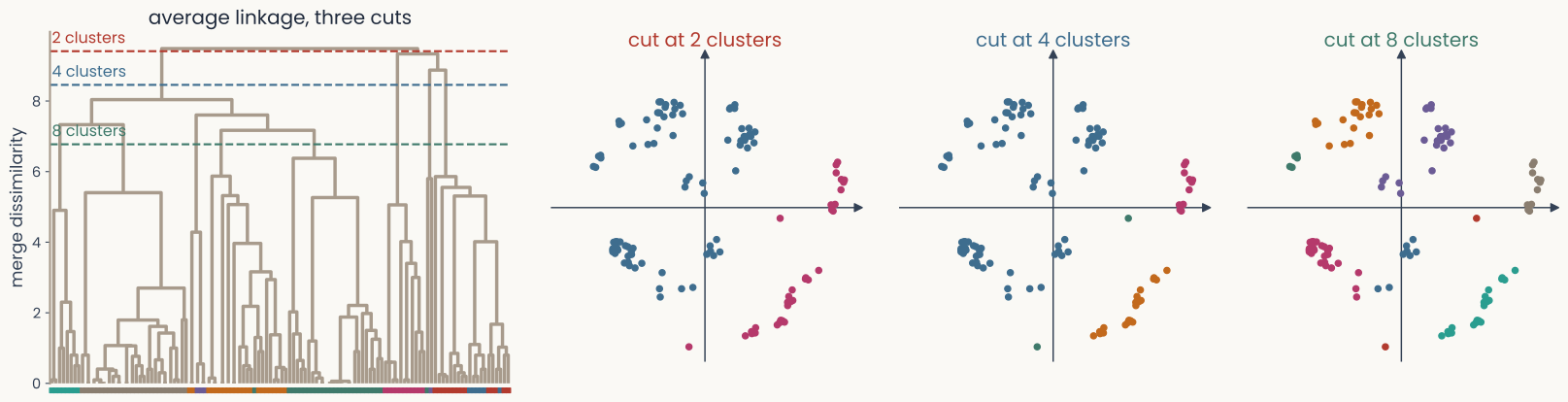
Left: the average-linkage dendrogram of the 120 animals with three dashed cut heights labelled 2, 4 and 8 clusters. Right: the MDS map of the same animals coloured by the clusters each cut produces; the 8-cluster cut nearly matches the eight taxa
A dendrogram is every clustering at once; you get groups by cutting it at a height. Cut low, many small clusters; cut high, few large ones. The method does not choose for you
Cut at 8: nearly the eight taxa (adjusted Rand index ). Cut at 2 or 4: not. is a choice you defend
Choosing where to cut the tree is parallel to choosing dimensions in MDS: both methods hand you a free parameter, and both are routinely reported as if it had been discovered rather than chosen
Same 120 animals and ratings · average linkage · map: metric MDS
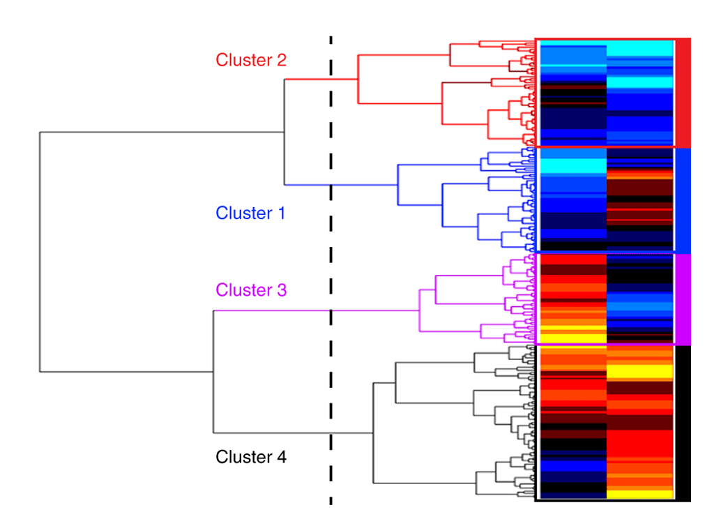
the dashed line is the cut; four colors are the four proposed groups
Over a thousand patients with depression, clustered on resting-state fMRI connectivity, cut into four "biotypes", each one claimed to predict who responds to which treatment.
Same algorithm as the last three slides. The arithmetic is not in question.
The biotypes did not replicate. Reanalysis found no evidence of genuine cluster structure in the data, and a tree comes back from any matrix, including one with no groups in it.
Whether the branches name something real is a separate claim, needing separate evidence.
Triangle inequality: . Two items can each be similar to a third on different features, and not at all similar to each other.
Nearest-neighbor restriction: in an -dimensional Euclidean space, a point can be the nearest neighbor of only a bounded number of others. Conceptual hierarchies break that bound: fruit is the nearest neighbor of many fruits at once, but an MDS map can only put it near two or three.
One correlation is a point estimate. Papers add three things; each has a catch.
Uncertainty. Bootstrap over stimuli (and over subjects when people made the RDM) for an interval on . One model beats another only if their intervals separate under the same resampling
Ceilings. Split-half is a proxy; toolboxes give a lower and an upper bound from how well each subject agrees with the group
Which pairs, which measure. depends on the stimulus set, and Spearman, Pearson, Kendall's or cross-validated distances can rank models differently on the same data. A result that holds under one measure is a result about the measure
What it does not show. Matching RDMs means the two systems order the pairs alike, not that they compute alike
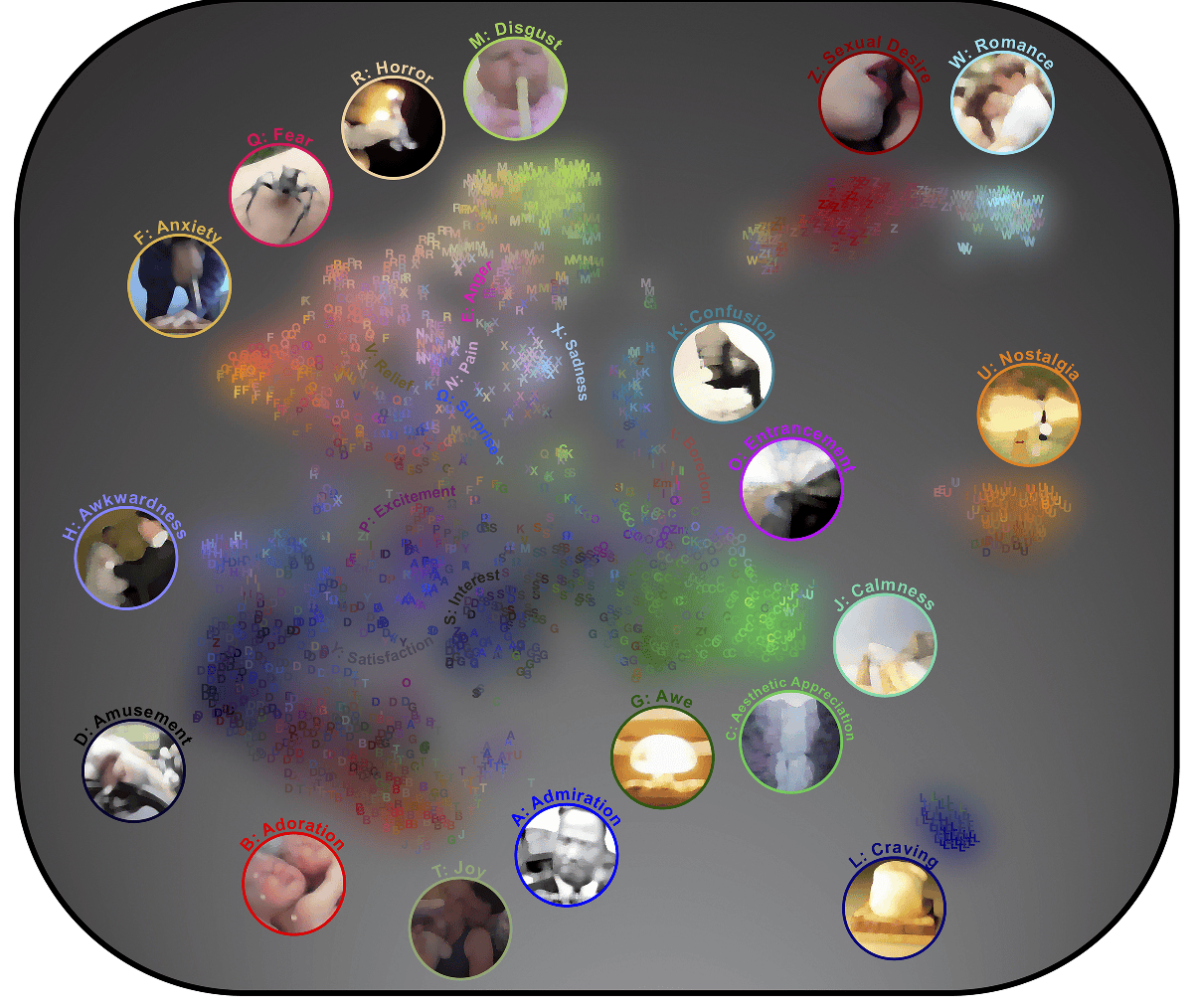
each letter is one video, colored by its dominant category
2,185 short videos rated by hundreds of viewers for what they felt. No stimulus dimensions, no recordings, judgments are the only input.
The structure that comes back needs 27 categories, not the textbook two, and they are joined by smooth gradients rather than gaps: anxiety shades into fear, fear into horror.
The 2-D layout here uses a nonlinear cousin of MDS, taught in a later lecture.