PCA & eigendecomposition
Reader-friendly version of the 60 lecture slides: the lecture content in normal flow, with figure descriptions and data tables where the figure carries data. Open the presentation.
Slide 1

PCA & eigendecomposition
Slide 2
Last time: comparing representational spaces
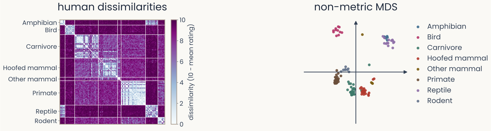
Left: the 120 animal photographs as a dissimilarity matrix built from people's ratings, blocked by animal category. Right: the two-dimensional map non-metric MDS recovers from that matrix, each point one photograph, coloured by category, with primates, birds and reptiles falling in separate regions
Open full-size figure- RDMs describe which stimuli a system treats as similar or different.
- Comparing RDMs lets us ask: do two systems organize the same stimuli similarly?
- MDS recovers a psychological space whose distances approximate the judged dissimilarities.
Slide 3
How many dimensions describe the variation?
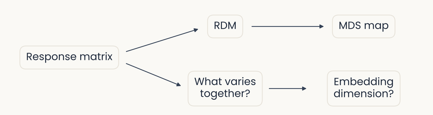
A response matrix linked to the RDM and MDS map from the previous lecture. Below it, the new questions: what varies together, and how many dimensions describe the variation (the embedding dimension)?
Open full-size figure- MDS summarized dissimilarities as coordinates in a psychological space. Now return to the response matrix: hundreds of measured dimensions—pixels, features or neurons—for each stimulus.
- If many responses vary together, their variation may occupy fewer dimensions: a smaller embedding dimension, the number of flat (linear) directions that hold most of it. How many are needed, and what is lost when we retain only some of them?
Slide 4
Can fewer coordinates capture the variation?
Which directions capture most of the variation, and what do we lose when we retain only a lower-dimensional description?
- Start with two pixels from the same photographs.
- Find a direction, project onto it, and reconstruct.
- Use the same operations to study images and neural responses.
Slide 6
Why look for a direction at all?
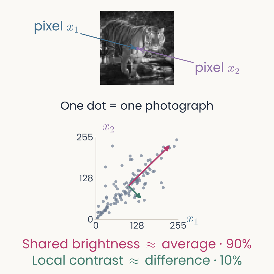
The same figure again, now with a long shared-brightness direction approximately corresponding to the two pixels' average and a short local-contrast direction approximately corresponding to their difference
Open full-size figure- Along the long arrow, both pixels brighten or darken together. Its weights are close to , so it behaves like their average and accounts for 90% of the variation.
- Along the short arrow, one pixel brightens as the other darkens. Its weights are close to , so it compares the two pixels and accounts for the remaining 10%.
- For this pixel pair, the two fitted directions are close to average and difference.
Slide 7
From the same dots to one distribution
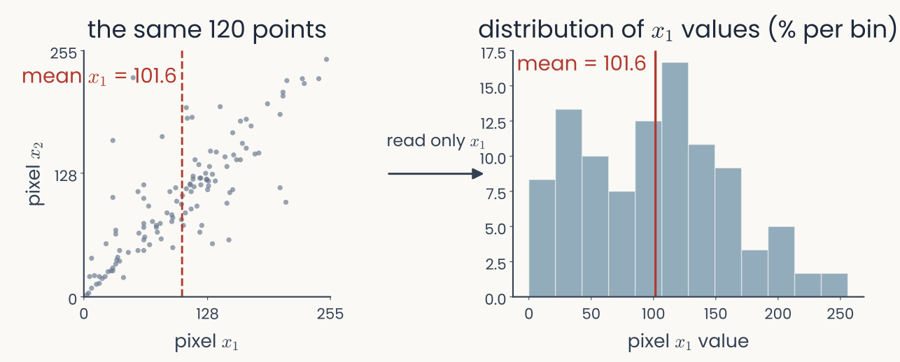
The same two-pixel scatter of dots from the previous slide appears on the left, with a vertical line at the mean x1 value of 101.6; an arrow labeled read only x1 leads to a histogram of those same 120 x1 coordinates with the identical mean marked
Open full-size figure- These are the same 120 dots. For the moment, read each dot's horizontal coordinate and set aside.
- The histogram is the distribution of those 120 values. Their mean is 101.6; their spread tells us how much this measurement varies across photographs.
Slide 8
From observed values to a Gaussian model
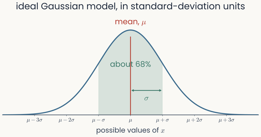
A complete symmetric Gaussian bell curve from three standard deviations below its mean to three above, with the mean marked, the interval of one standard deviation shaded, and approximately 68 percent written inside it
Open full-size figure- The previous histogram showed observed pixel values. This is an idealized reference model, not an assumption today's method requires.
- A Gaussian is smooth and bell-shaped. Its mean gives the center and its standard deviation gives the spread; about 68% lies between and .
Slide 9
The Gaussian model in two dimensions
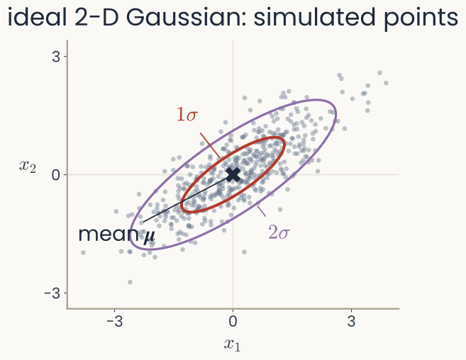
Five hundred points sampled from a two-dimensional Gaussian, forming a tilted ellipse of points centered at the mean, with one- and two-standard-deviation elliptical contours
Open full-size figure- Each simulated point contains two measurements, . These are draws from the model, not the 120 photographs.
- The mean becomes a mean vector , the center of the points; the covariance matrix describes their width, elongation and tilt.
- PCA will find the directions along which the ellipse is longest and shortest.
Slide 11
Where are the points, and how do they spread?
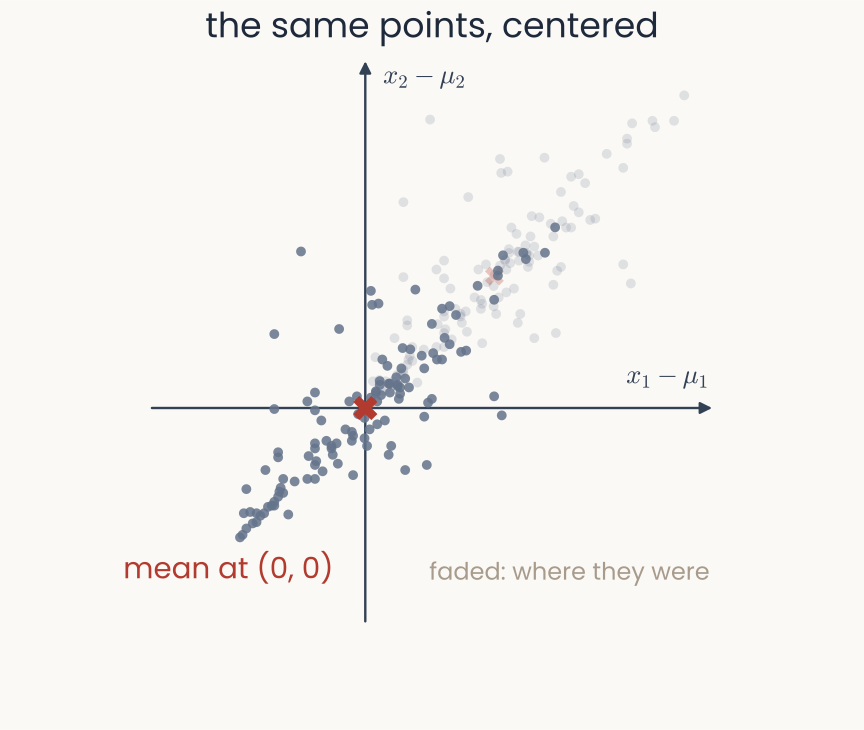
The same points after subtracting their mean, now sitting at the origin with the axes crossing through the middle of the points
Open full-size figure- So subtract the mean from every point: . This is centering, and it slides the points until their centre sits at the origin.
- PCA describes variation around the mean.
- A negative centered value means “darker than this pixel’s average,” not a negative raw intensity.
Slide 12
Centering, in code
mean = features.mean(axis=0)     # (D,) mean response across stimuli, for each coordinate
centered = features - mean        # (N, D) each stimulus response minus the mean response
featuresis the response matrix from the first lectures: one row per stimulus (images here), one column per coordinate.- The mean is a vector with one entry per coordinate. Subtracting it from every row leaves each column summing to zero.
- Keep the mean. PCA works on differences from it, and reconstruction adds it back.
Slide 13
Covariance: do the deviations go together?
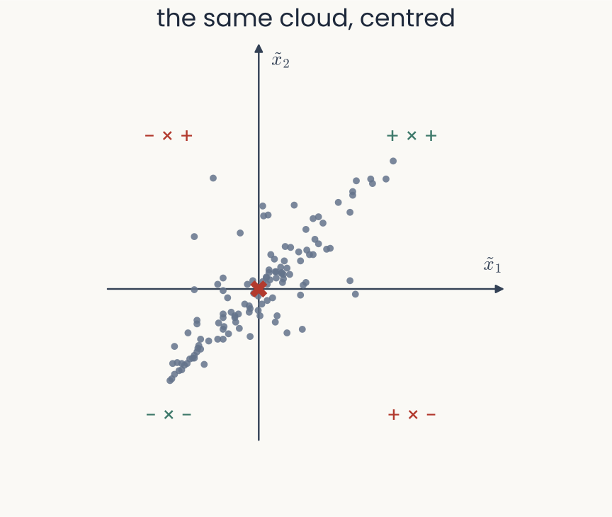
The same centered pixel points and coordinate frame as before, with axes x1 minus mu1 and x2 minus mu2. Signs in each quadrant show whether multiplying the two deviations gives a positive or negative result.
Open full-size figure- These are the same centered responses: and . Same signs give a positive product; opposite signs give a negative product.
- Covariance is their average product:
. - Pearson correlation is covariance measured in standard-deviation units:
.
Slide 14
The covariance matrix
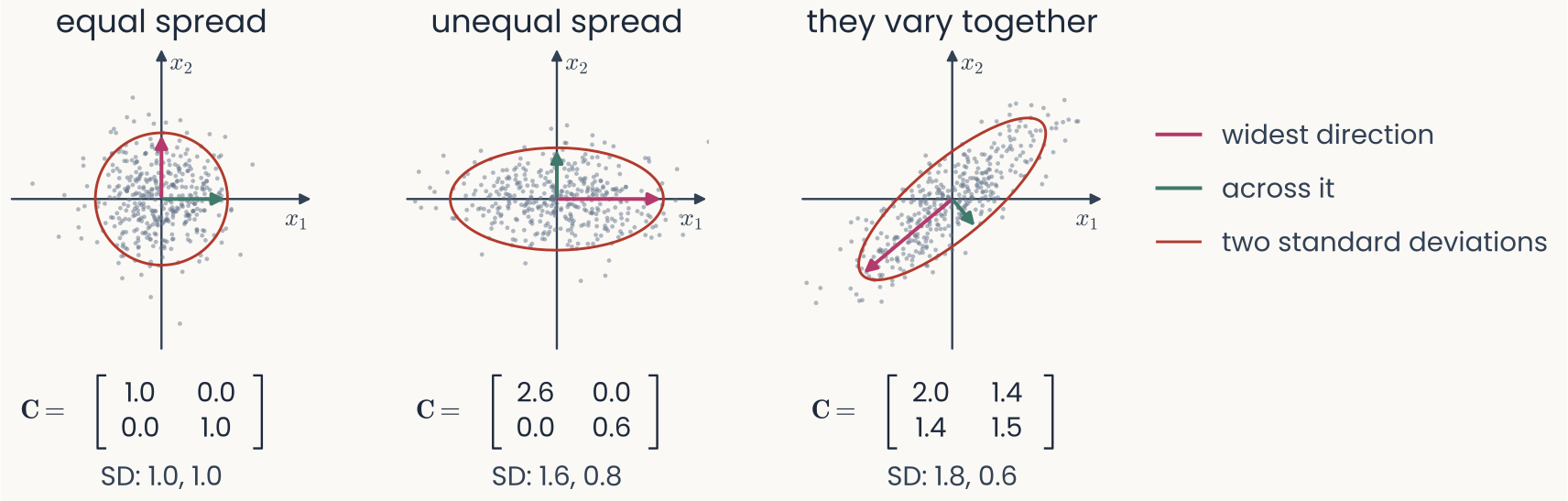
Three sets of two-dimensional points side by side, each with its two-by-two covariance matrix printed underneath: a round set with equal spread in both directions, an ellipse stretched along the horizontal axis, and a tilted ellipse that runs diagonally
Open full-size figure- In , the diagonal contains the variances. The same covariance appears on both sides of the diagonal because .
- Geometrically summarizes the points’ spread and orientation: round, an ellipse, or an ellipse tilted because the two vary together.
- The ellipse's long direction is its direction of greatest variance.
Slide 17
Projection onto a unit direction
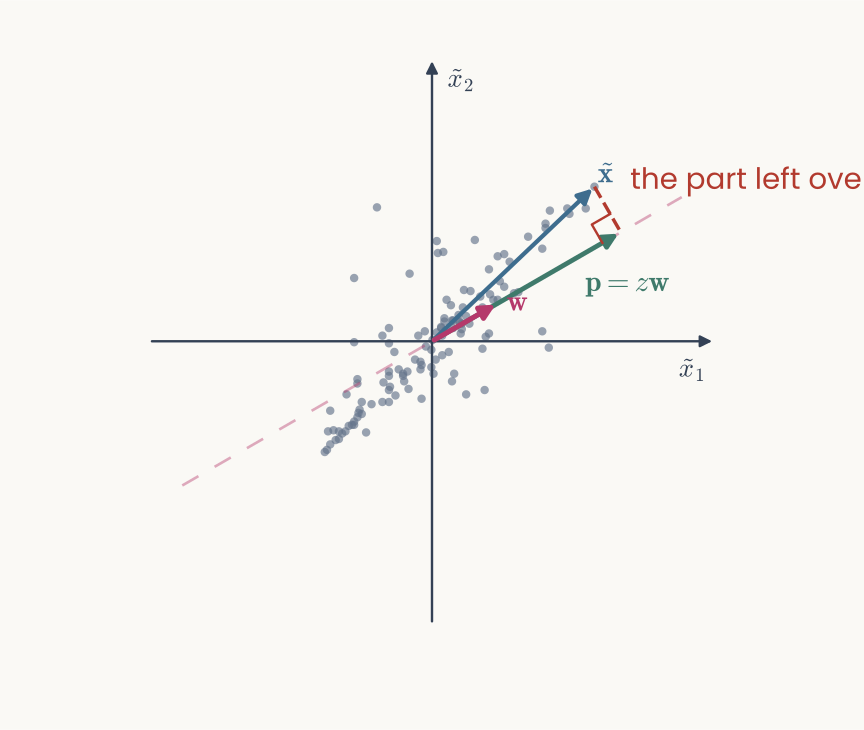
The two neighboring pixels, centered, with one point marked as the centered vector x tilde, a magenta line through the origin along the unit direction w, and the construction of the projection
Open full-size figure- The foot of that perpendicular is : the part of that lies along .
- Here : two coordinates become one score, .
- More generally, retained directions replace coordinates with scores.
Slide 18
A direction keeps part of the spread
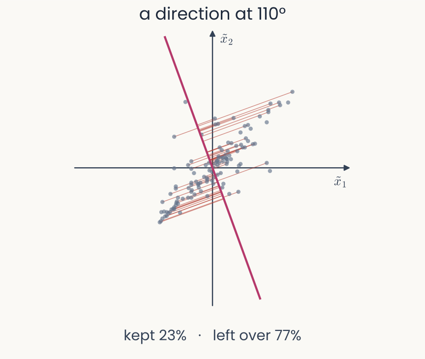
The two neighboring pixels again, a direction drawn at 110 degrees, and a short red segment from every point to the line showing what that direction does not capture
Open full-size figure- Project every point onto some direction. The red segments are what is left over: the part each point keeps to itself.
- At this angle the direction keeps 23% of the total spread and leaves 77% over.
Slide 19
Turn it until the leftovers are smallest
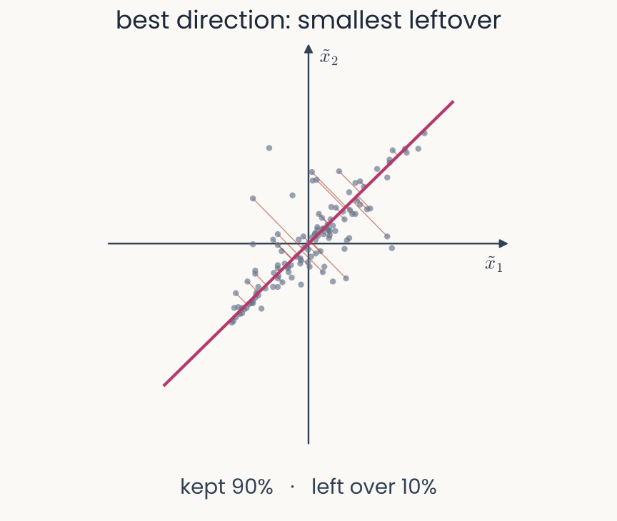
The same points with the direction turned to 44 degrees, lengthwise through the points, and the red segments now short
Open full-size figure- Turn the direction until those segments are as short as possible: here at 44°, lengthwise through the points.
- Now it keeps 90% and leaves 10%.
Slide 20
Spin the direction yourself
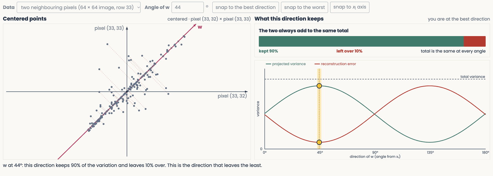
The direction-spinner demo with the direction at its best angle of 44 degrees: the centered points with the leftover segments drawn from each point, a bar showing 90 per cent kept against 10 per cent left over, and a sweep of both quantities against the angle with the smallest-error angle marked in gold
Open full-size figure- Before turning the direction, predict which direction leaves the smallest error.
- Projected variance and squared reconstruction error add to a fixed total. Maximizing one minimizes the other.
Slide 21
From turning the line to a calculation
The familiar centered pixel points with the best direction at 44 degrees, retaining 90 percent of the variance and leaving the smallest residual
Open full-size figure- For a unit direction , each centered response has one score: .
- Across all stimuli, those scores have variance
- The best direction is the that makes this variance largest. The covariance matrix lets us find it without searching every angle.
Slide 22
The covariance matrix changes a direction
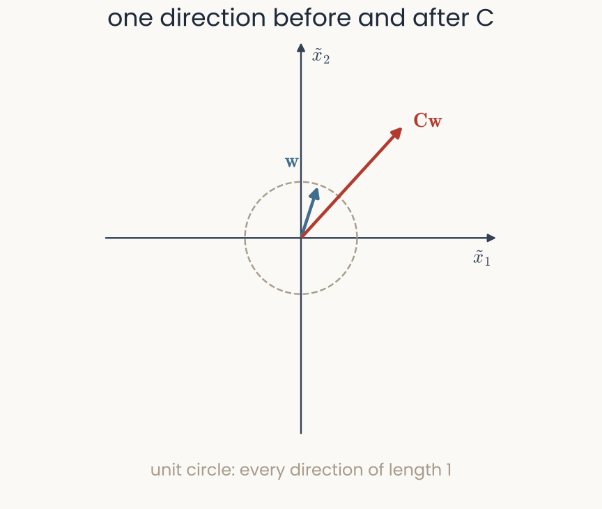
A unit direction w and the vector Cw produced when the covariance matrix acts on it; Cw has a different length and orientation
Open full-size figure- The blue vector is one possible direction through the response space.
- Multiply it by the covariance matrix: is the red vector.
- Usually, the red vector has a different length and points in a different direction.
Slide 23
Most directions turn
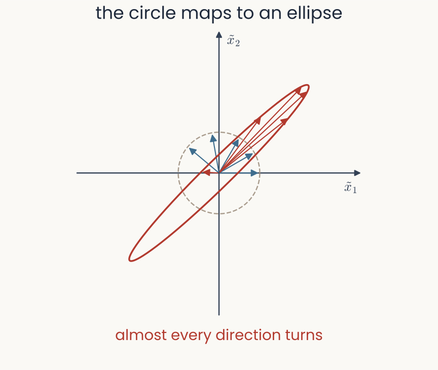
The unit circle with several directions and their transformed vectors; their tips trace an ellipse and almost every vector changes orientation
Open full-size figure- Apply to every direction on the unit circle. The transformed tips trace an ellipse.
- Almost every direction comes out turned as well as rescaled.
Slide 24
Eigenvectors are directions that do not turn
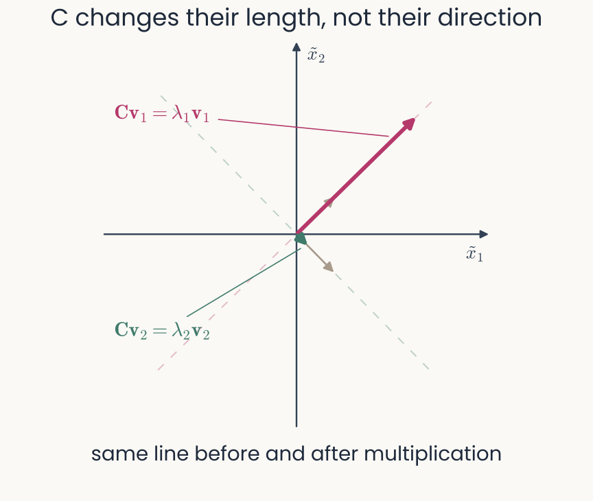
Two special directions shown before and after multiplication by the covariance matrix; each transformed vector remains on the same dashed line
Open full-size figure- For most vectors, points in a different direction from .
- An eigenvector is special: changes its length but leaves it on the same line.
- The amount of scaling is its eigenvalue :
Slide 25
An eigenvalue gives variance along its eigenvector
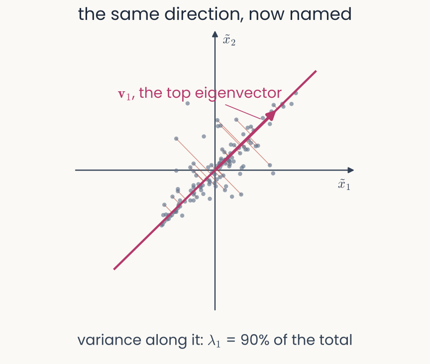
The same centered pixel points and the same 44-degree line as the best-direction slide, now with the eigenvector v1 drawn along it as an arrow and the variance along it given as 90 percent of the total
Open full-size figure- Put into the variance formula, then replace by :
since has length 1.
- The largest eigenvalue identifies the direction with the most variance. Here it is the same 44° direction found by turning the line.
- Ranked by eigenvalue, these directions are the principal components. The first is PC1; computing them is principal component analysis (PCA).
Slide 26
PCA = eigendecomposition of
Covariance (centered, samples): (code divides by ; same eigenvectors)
Eigendecomposition (orthonormal ):
- Principal directions = eigenvectors of .
- Variance along = .
- , the eigenvector with the largest eigenvalue.
Slide 27
From a line to a plane
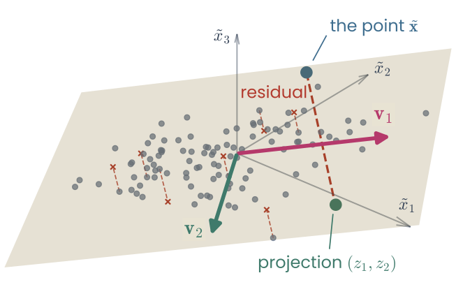
A three-dimensional set of points near a plane spanned by two principal directions; one point and its projection on the plane
Open full-size figure- In this picture, measured coordinates and we retain perpendicular directions.
- The two directions define a plane; each centered point gets two scores, .
- Keeping all directions changes coordinates without losing information.
- Keeping projects each point onto a lower-dimensional flat (linear) subspace: a line, a plane, or its analogue in more dimensions.
Slide 28
The new coordinates are the PC scores
The same three-dimensional centered points and retained plane; the highlighted point projects to a location with coordinates z1 and z2 in the principal-component basis
Open full-size figureFor one stimulus, take its dot product with each retained direction:
- gives weights on the original measurements.
- The score is this stimulus's coordinate along that direction.
- Keeping directions gives the point scores.
Slide 29
The same points, in the new coordinates
A three-dimensional set of points lying close to a plane spanned by v1 and v2, with axes x-tilde 1, 2 and 3; one point off the plane and its projection
Open full-size figure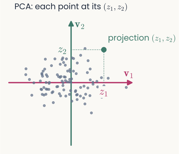
The same 100 points drawn in two dimensions at their scores z1 and z2 along v1 and v2; the projected point is marked in green
Open full-size figure- Left: points in the original measured coordinates . Right: the same points at their scores : the PCA embedding.
- The green point is the same stimulus in both. Its distance from the plane, the dashed red residual, is what the 2-D map leaves out.
Slide 30
Reconstruction: the way back
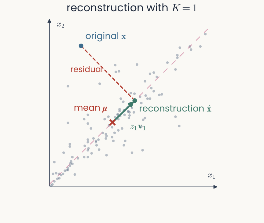
The raw two-pixel points with their mean, one original point, and its reconstruction formed by adding the score-weighted first principal direction to the mean; the residual joins the reconstruction to the original
Open full-size figure- Return to the original measurement coordinates and start from the mean.
- Add each retained direction, weighted by the image's score:
- The residual is the difference between the original and reconstructed measurements.
Slide 31
What do we lose when we keep fewer components?
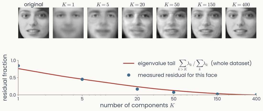
Top: one face reconstructed with K equal to 1, 5, 20, 50, 150 and 400 components, from a blurry near-average to the exact original. Bottom: the residual fraction for this face at each K as dots, compared with the eigenvalue tail computed from the whole dataset
Open full-size figure- PCA on the pixels of 400 faces: keeping more components adds detail and reduces reconstruction error.
- A residual fraction of 0 means exact reconstruction; larger values mean more of that face was left out.
- Dots: this face. Curve: the discarded variance across all 400 faces, which need not equal one face's error.
Slide 32
How many components? The scree plot
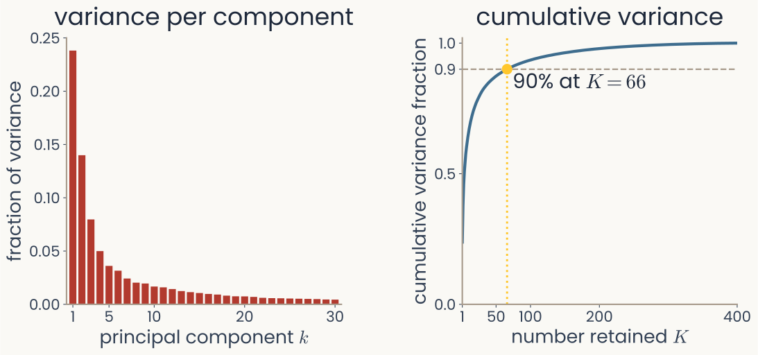
Scree plot for the 400 Olivetti faces: the variance fraction carried by each principal component, and the cumulative fraction
Open full-size figure- These are the same 400 faces. The left panel shows the variance fraction carried by each PC.
- The cumulative curve answers how many PCs are needed to retain a chosen fraction, such as 90%: the embedding dimension at that threshold.
- A variance threshold sets a reconstruction budget. It does not establish performance on a task.
Slide 33
PCA in scikit-learn
from sklearn.decomposition import PCA

pca = PCA(n_components=K, svd_solver="full")
Z = pca.fit_transform(X)       # X: (N, D)  ->  Z: (N, K)
fraction = pca.explained_variance_ratio_
directions = pca.components_  # one principal direction per row
- Score: a stimulus's coordinate along a principal direction.
fit_transformcenters each feature across stimuli. It does not z-score them (divide each by its standard deviation).- SVD computes the PCA directions and variances from the centered data without explicitly forming its covariance matrix.
Slide 34
Can these directions help explain a neuron?
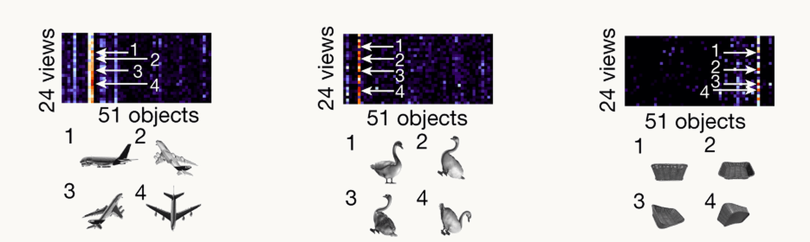
Three example IT cells from Bao and colleagues, each shown as a 24-view by 51-object response matrix with four views of the cell's preferred object picked out and shown underneath: an aeroplane, a swan and a basket
Open full-size figure- Inferotemporal (IT) cortex is part of the primate visual pathway involved in object recognition.
- Each matrix shows one cell's responses: 51 objects × 24 views. A bright column means strong responses across views of one object.
- Can a space derived from a network's responses help organize these preferences?
Slide 35
Build an object space from network responses
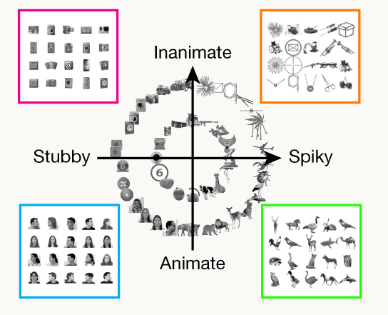
Bao et al.'s schematic of the AlexNet object space: stimulus images arranged in the plane of the first two PCs, in four colored groups
Open full-size figure- Present the 1,224 images to AlexNet and collect responses from fc6, a late network layer.
- Run PCA on those response vectors. In the paper, 50 components account for 85% of the variance.
- The picture is a schematic of the first two PCs, arranged for legibility rather than a raw scatter plot.
- “Stubby–spiky” and “animate–inanimate” are proposed interpretations of those directions. They need testing.
Slide 36
Test whether a direction predicts a response
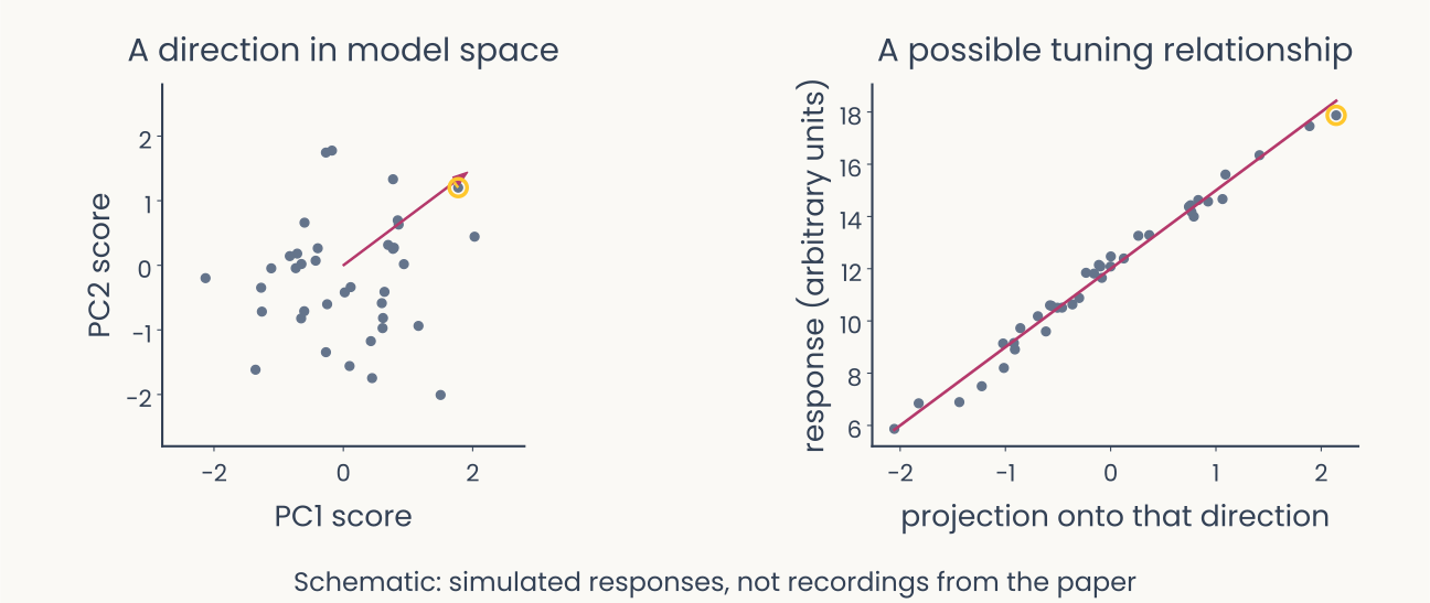
Schematic simulated example: projecting points in model space onto a direction gives a scalar related to a simulated neural response
Open full-size figure- The gold ring follows one image from its position in model space to its measured response.
- Choose a direction using training images, then ask whether each image's projection predicts the cell's response on held-out images, which were not used to choose it.
- The preferred direction can combine several PCs; it need not coincide with PC1 or PC2.
Slide 37
Neural preferences occupy different regions
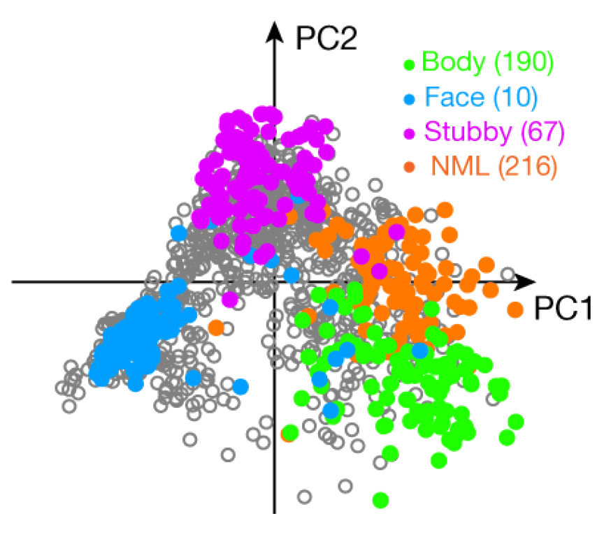
Grey stimulus points in the PC1-PC2 plane with four colored groups of points — the preferred images of four IT patch systems — landing one per quadrant
Open full-size figure- Grey circles are stimuli in the network-derived PC plane.
- Colored points are images that strongly activate four IT systems. NML is the network Bao et al. found in IT's "no man's land", cortex that no earlier localizer had assigned a category; the numbers in parentheses count recorded neurons.
- Different IT systems prefer different regions of the model space. A separate analysis tests whether a neuron's response varies with its projection along a direction.
Slide 38
Use the space to make a new prediction
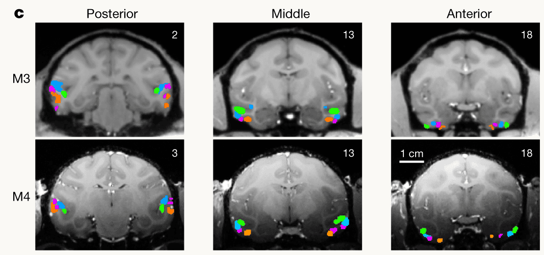
Published coronal fMRI maps from two monkeys, showing the four networks at posterior, middle and anterior IT; magenta marks the predicted stubby-object network
Open full-size figure- The object space predicted a system responding to stubby, inanimate objects.
- fMRI located it (magenta); targeted recordings confirmed the object preferences.
- A description of a representation can guide a new experiment.
Slide 39
The measurement scale changes PCA
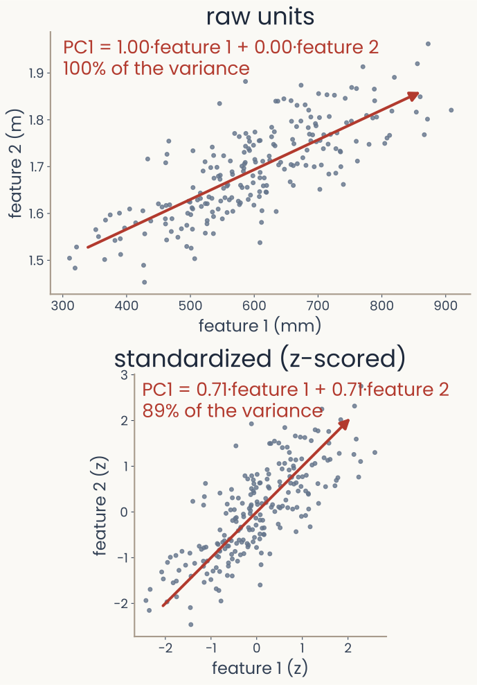
The same correlated points twice. Top, in raw units with feature 1 in millimetres and feature 2 in metres, PC1 equals 1.00 times feature 1 plus 0.00 times feature 2 and carries 100 percent of the variance. Bottom, after z-scoring, PC1 is 0.71 times each feature and carries 89 percent
Open full-size figure- PCA maximizes variance, so a feature measured in millimetres dominates one measured in metres: in raw units PC1 is and the second feature is invisible.
- After z-scoring each feature (subtract its mean, divide by its standard deviation), PC1 is and recovers the diagonal structure the two features share.
- Standardize when the units are not comparable. When they are comparable and the variances differ for real reasons, standardizing changes the relative weighting of features; it is a modelling decision, not a default.
Slide 40
Most variance need not mean most useful
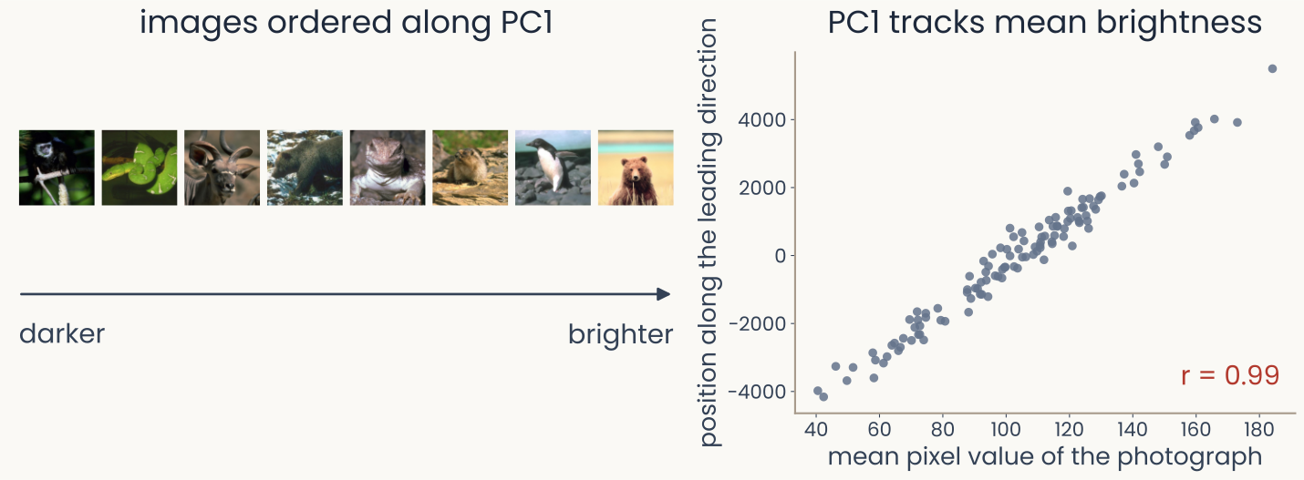
Left: the 120 photographs laid out along the leading direction of their pixel coordinates, running from dark pictures to bright ones with animals of different categories interspersed. Right: position along that direction plotted against the mean pixel value of each photograph, an almost perfect straight line, r equals 0.99
Open full-size figure- The largest direction in the 120 photographs carries 29% of the variation and is strongly related to overall brightness: ordered along it they run dark to bright, different categories interspersed.
- Would this direction help distinguish the animals? This plot alone cannot answer.
- PCA ranks directions by variance; the task determines what is useful.
Slide 41
Which direction would you keep?
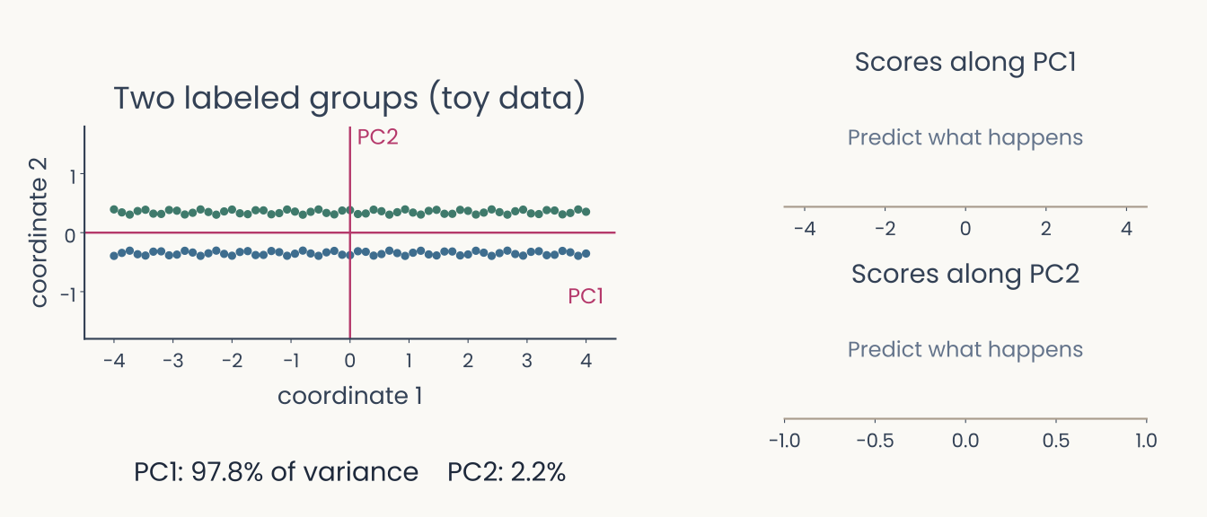
Toy classes with a high-variance horizontal direction and low-variance vertical separation; projection panels ask for a prediction
Open full-size figure- The groups vary mainly from left to right. Their labels differ from top to bottom.
- Which direction would best reconstruct the points?
- Which direction would best distinguish the groups?
Slide 42
Low variance can still separate the groups
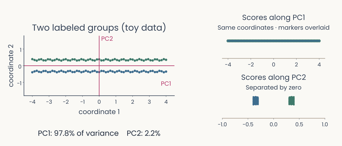
Toy classes with a high-variance horizontal direction and low-variance vertical separation; PC1 scores overlap while PC2 scores separate the classes
Open full-size figure- PC1 retains 97.8% of variance, but both groups have the same PC1 coordinates.
- PC2 retains 2.2%, yet a threshold at zero separates the groups.
- Variance measures spread. Task relevance depends on what we want to distinguish.
Slide 43
What PCA provides
The two neighboring pixels again, with the direction that retains about 90 percent of their variance
Open full-size figure- PCA replaces many measurements with ordered scores and tells us how much variance each direction retains.
- Those scores support reconstruction and can connect a model representation to neural responses. In the Bao study, that connection helped motivate a new experiment.
- PCA describes variation. A separate test establishes what the variation is useful for.
Slide 44
What if the variation follows a curve?
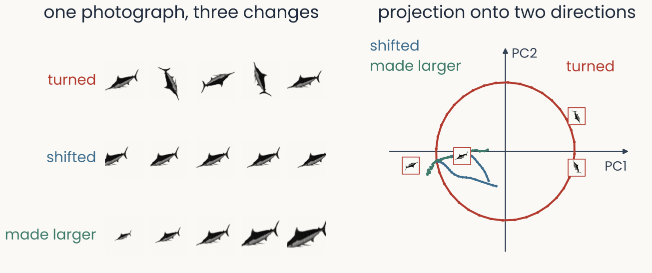
Rotated, shifted and resized versions of an image projected into two PCA directions; rotation traces a closed curve
Open full-size figure- Changing one stimulus parameter can trace a curved path in a large response space.
- Even one varying parameter can require two linear coordinates when the path bends back on itself.
- PCA approximates data with a flat subspace.
- Next: nonlinear maps, and how to check what their geometry preserves.
Slide 45
Further reading for the research trail
- Bao et al. (2020): object-space directions and IT responses. Nature
- Chang & Tsao (2017): face-space directions and individual neurons. Cell
- Turk & Pentland (1991): eigenfaces. J. Cogn. Neurosci.
- DiCarlo & Cox (2007): untangling object representations. Trends Cogn. Sci.
- Stringer et al. (2019): a structured, high-dimensional neural spectrum. Nature
Trail entry: pick any paper cited in a lecture so far, read it, and post four to six sentences on Ed under Research trail — what it did, and what surprised you or what question it left you with. Reply once to a classmate. Next deadline Fri 9/25, best three of four entries count.
Slide 46
Minute paper
Submit on Canvas → Minute papers → Minute Paper 4.
Write three brief points in your own words:
- Why do we center the data before finding the principal directions?
- Something you do not yet understand, or a question still open
- Another idea you found interesting, and why it matters for brains, behavior or AI
Credit for a thoughtful attempt, not for being correct.
Slide 47
Appendix: examples and implementation details
Additional examples, the PCA/SVD implementation, and reference material for the assignments.
Slide 48
One direction was not enough
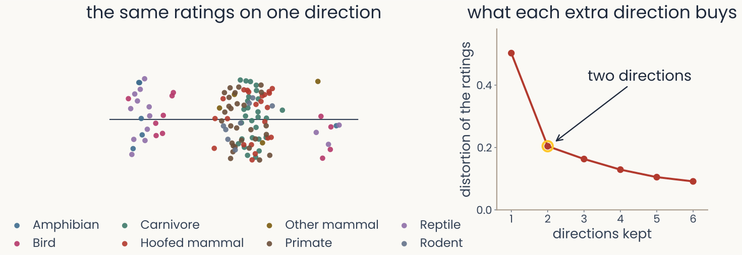
Left: the same 120 photographs placed on a single direction, coloured by animal category, with the categories piled on top of one another. Right: the distortion of the ratings plotted against the number of directions kept, falling steeply from one to two and then flattening out
Open full-size figure- Fit the same ratings on one direction and the categories pile up: the distances in the fit no longer match the judged dissimilarities.
- A second direction removes most of that distortion. A third and a fourth remove very little. Two directions greatly improve the fit, but some distortion remains.
Slide 49
How far does the dependence reach?
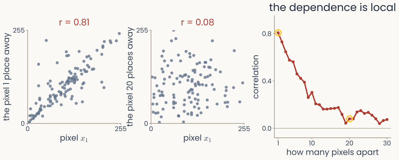
Three panels. Left: a pixel plotted against its immediate neighbour across the 120 photographs, the points hugging the diagonal at r equals 0.81. Middle: the same pixel against the one twenty places away, points with no visible trend at r equals 0.08. Right: the correlation plotted against separation, falling steeply over the first few pixels and flattening near zero
Open full-size figure- The same pixel-pair computation, at larger separations: one pixel against another, across the same 120 photographs.
- Next door, the two pixel values strongly covary. Twenty pixels apart, they barely covary.
- Neighbouring measurements are strongly dependent, and the dependence is local.
Slide 50
PCA in code: two routes to the same answer
centered = features - features.mean(axis=0)

# Route 1: eigendecomposition of sample covariance
C = np.cov(centered.T)
lam, V = np.linalg.eigh(C)                 # ascending order
lam, V = lam[::-1], V[:, ::-1]             # descending order

# Route 2: SVD, without forming C
_, s, Vt = np.linalg.svd(centered, full_matrices=False)
lam2 = s**2 / (len(centered) - 1)
V2 = Vt.T                                # directions as columns
Z = centered @ V2[:, :K]                   # (N, K) scores
- Use
eigh, noteig: is symmetric, so the eigenvalues are real andeighis faster and stabler. It returns them ascending, so the reversal is not optional. - Prefer route 2. Forming costs memory; for a color image and would be ~309 GB in float64. SVD never builds it. Sign is arbitrary: and are both valid; Assignment 2's helper fixes it so the largest entry is positive.
Slide 51
Eigenfaces
PCA on 400 faces, and a classic approach to face recognition.
Slide 52
PCA as compression: eigenfaces
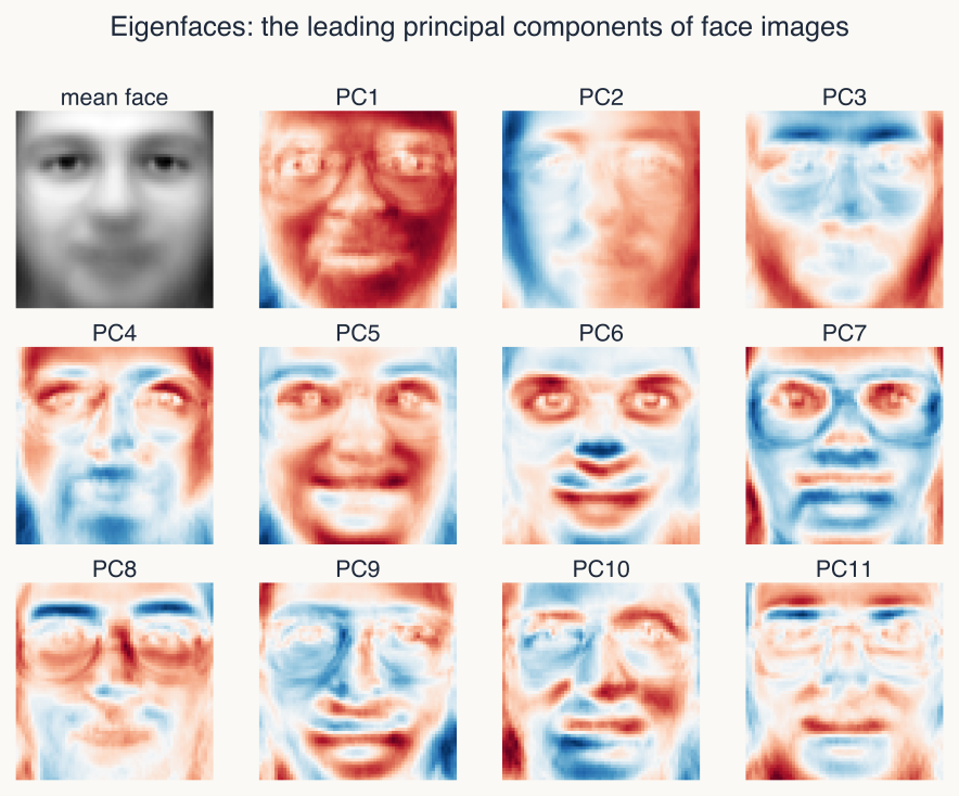
Grid of the mean face and leading eigenfaces, with opposing signs shown in red and blue
Open full-size figureStack face images as vectors and run PCA → the leading eigenvectors are eigenfaces: ghostly, face-like basis images, one direction in pixel space each.
Slide 53
Face space
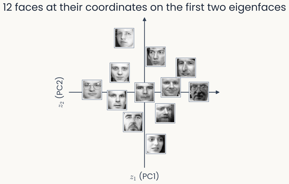
Twelve face photographs placed on a plane at their coordinates along the first two eigenfaces, z1 on the horizontal axis and z2 on the vertical
Open full-size figure- 400 face images ( pixels, so ), PCA on the centered pixels, and twelve of the faces drawn at their coordinates on the first two eigenvectors.
- Two numbers per face instead of 4,096. They carry 24% and 14% of the variance: a coarse, lossy summary, but already one in which lighting and head pose vary smoothly across the plane.
- This is a face space: every face is a point, and nearby points are faces that look alike to the two leading eigenfaces. The preceding slide shows those eigenfaces as images.
Slide 54
A face = mean + a few eigenfaces
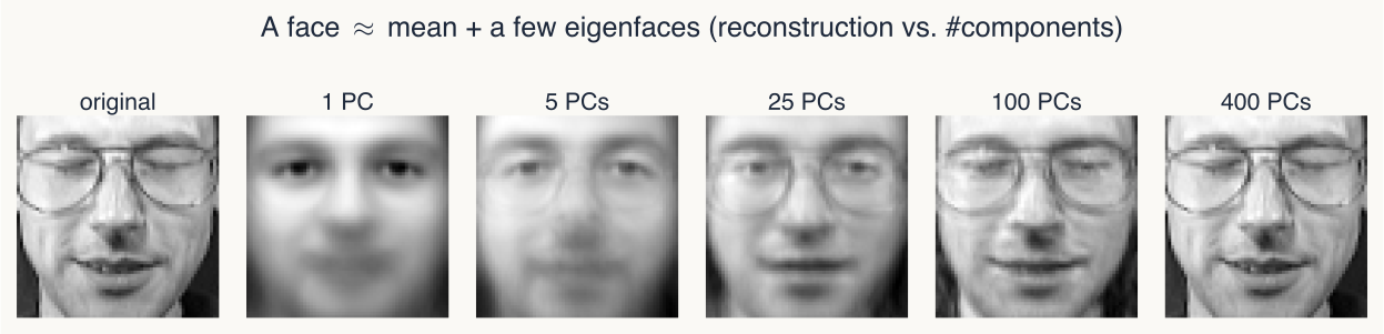
A face reconstructed using 1, 5, 25, 100 and 400 components, beside the original image
Open full-size figure- These faces can be approximated by the mean face plus a weighted sum of eigenfaces. More components add finer detail.
- Turk & Pentland used the coefficients for recognition: a new face is matched to the stored face with the nearest coefficients.
Slide 55
Mix your own face
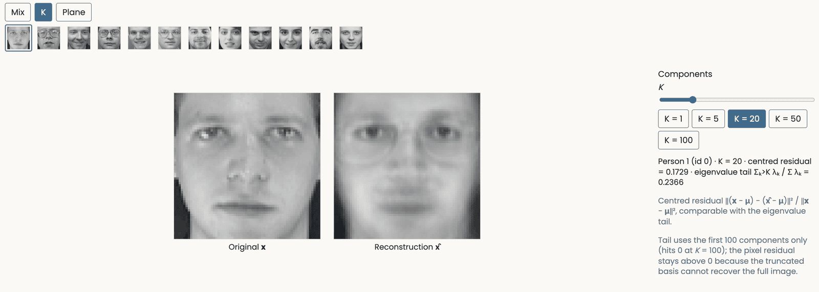
The eigenface mixer's K tab: one Olivetti face beside its reconstruction from the first 20 components, with the residual fraction and the eigenvalue tail printed
Open full-size figure- Each slider sets one coefficient in mean + weighted eigenfaces.
- Set a coefficient to zero to remove that direction’s contribution.
Slide 56
Two views, one answer
- Maximize the variance of the projections:
- Minimize the squared reconstruction error:
- These are the same problem: total variance is fixed, so whatever the projection captures, the residual loses. Both are solved by the top eigenvector of .
- For retained PCs, the average squared fitting-data reconstruction error is (using covariance divided by ).
- Connection to MDS: classical MDS on a Euclidean dissimilarity matrix returns the PCA coordinates up to an orthogonal transformation of the centered data.
Slide 57
PCA as decorrelation & whitening
- Project onto the eigenbasis and the new coordinates are uncorrelated: the covariance becomes diagonal. For positive eigenvalues, rescale each retained direction by and you get whitening: zero correlation, unit variance.
- Why analysts reach for it:
- remove redundancy between measured dimensions before modeling
- decorrelate inputs, without assuming the resulting features are independent
- compress by dropping directions; whether this denoises depends on what they contain
Slide 58
What do the components look like?
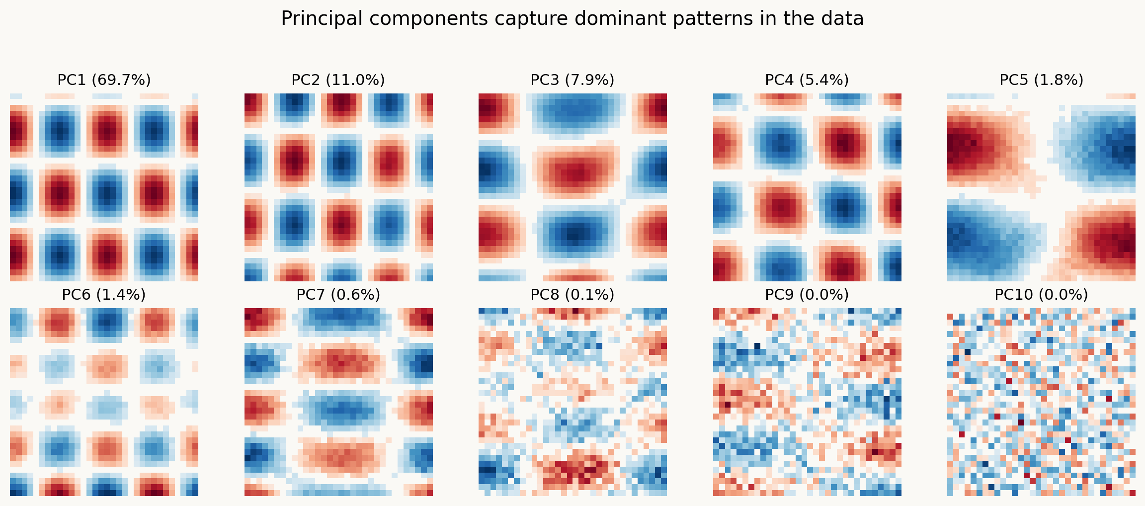
Principal components of synthetic image patterns, shown as red and blue signed weights: structured patterns dominate early components and noise appears in later ones
Open full-size figure- Each eigenvector is a vector in the original space, so each PC unrolls into a picture. Here the inputs are synthetic patterns: early components recover structured variation; later ones contain little variance.
- The components can be read as weights on the original variables, then tested for what they capture.
Slide 59
The rainbow cortex is three numbers per voxel
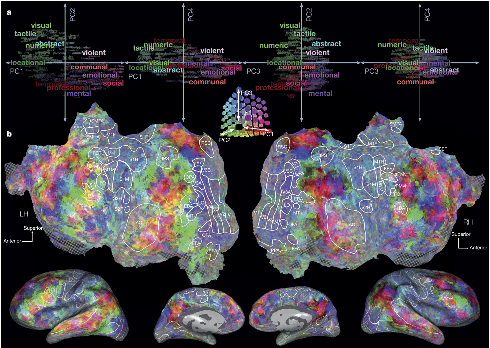
Panels from Huth et al. showing word-related features above cortical surfaces, where every voxel is colored by its first three PCA coordinates (red for PC1, green for PC2, blue for PC3), producing a smooth rainbow map across cortex
Open full-size figure- Over two hours of narrated stories, one regression per voxel: every voxel gets a vector of weights on word-related features, and cortex is one more matrix.
- PCA on it, keep three components, color each voxel by its coordinates: PC1 → red, PC2 → green, PC3 → blue. The palette is the projection .
Slide 60
PCA finds flat subspaces
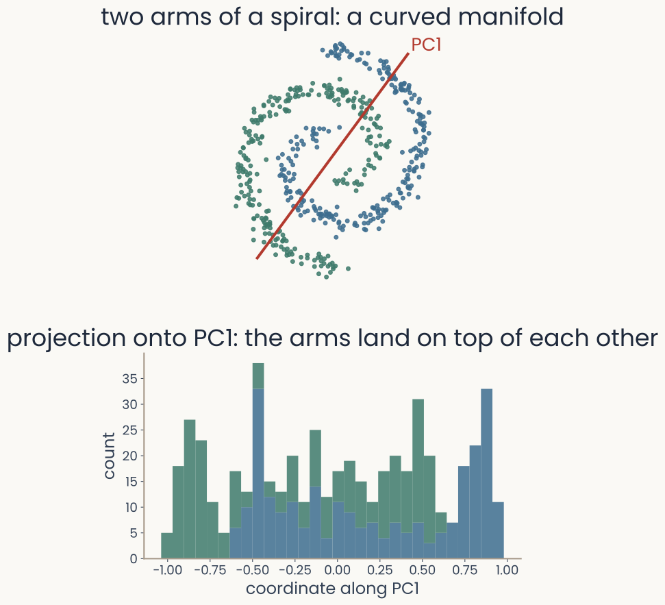
Top: two interleaved spiral arms, one blue and one green, with the PC1 line drawn through them. Bottom: the histogram of the coordinates along PC1, where the two arms overlap almost completely
Open full-size figure- If the data lie on a curved manifold, a smooth curved surface (a spiral, a Swiss roll, a torus), a low-dimensional linear projection can fold distinct regions onto each other.
- Two points far apart along the manifold can land on top of each other after projection: the two arms are perfectly distinct in the plane and inseparable along PC1.
- t-SNE and UMAP construct nonlinear maps emphasizing local relationships. Their displays can distort global structure and need their own checks.