Geometry of neural representations

Slide 2

Where we are

Where we are — table
Lecture	Takes in	Recovers	Why it matters
MDS	an RDM, e.g. people's similarity ratings	a map: the psychological space	a mental space measured from judgments alone
PCA	the response matrix (images × neurons)	the directions of largest variance, the principal components	how many directions hold most of the variance
t-SNE, UMAP, Isomap	the response matrix	a 2-D map that keeps neighbors on a curved shape (a manifold)	whether one object's views stay together

Two inputs: an RDM (one number per pair of images) or a response matrix (one per image and neuron).

Slide 4

Today: two questions

The data: the response matrix (images × neurons) of a population of neurons
Two questions about a recorded population:
1. How many dimensions does a population of neurons use?
2. What can another neuron read from the responses?
How: (1) count directions with PCA's eigenvalues, summed up by the participation ratio; (2) fit a linear readout, a boundary between groups of images, scored on new images
Next lecture: we finish question 2 (shattering, CCGP), then compare two representations

Claims such as "V1 is high-dimensional" or "IT encodes animacy" rest on these computations.

Slide 5

How many dimensions does a population of neurons use?

Slide 6

Why count dimensions?

Each image's response is one point in the neural state space: one axis per recorded neuron
Hubel & Wiesel (course introduction): V1 neurons prefer different orientations at different positions. There are only so many orientations, so many neurons may repeat one another
Mouse V1, ~10,000 neurons: how many independent directions do the responses use?
GPT-2, 768 units of layer 7: how many directions do the days of the week use?

With heavy redundancy, the population uses far fewer dimensions than neurons recorded.

Slide 7

Three measures of dimension: GPT-2

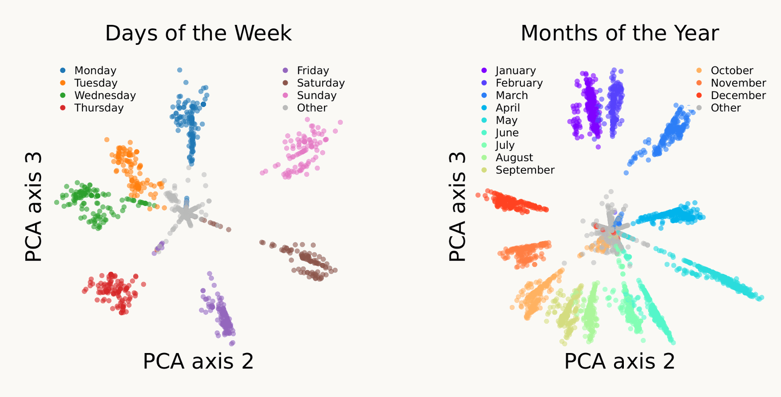
Two panels from GPT-2-small, layer 7, projected on principal components 2 and 3, with a wide gap between them. Left, the representations of the seven days of the week form a ring of colored clusters in calendar order, Monday to Sunday. Right, the twelve months form a ring in calendar order, January to December
Open full-size figure

Reproduced from Engels et al. (2025), Fig. 1 (CC BY 4.0): GPT-2, layer 7

Ambient 768 units · embedding 2: 90% of the variance fits in a plane · intrinsic 1
t-SNE or UMAP on these responses would draw the ring: they estimate the manifold
Each measure answers a different question, so none is the dimensionality (Perich 2026)

Engels et al. ICLR 2025 · Perich The Transmitter 2026

Slide 9

Rank: how many directions the points span

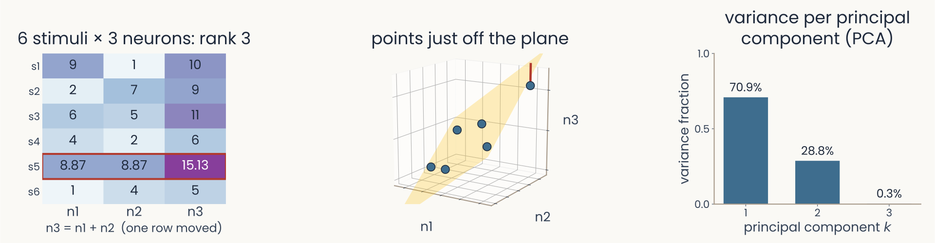
The same three panels with one stimulus moved off the plane: its value for neuron 3 no longer equals the sum of neurons 1 and 2, the point sits off the gold plane in the 3-D view, and the third principal component now has a small nonzero bar
Open full-size figure

Toy data, computed

Rank = number of directions with nonzero variance = number of principal components (PCA) with nonzero variance. Neuron 3 = neuron 1 + neuron 2, so here rank 2: a plane
One stimulus off the plane: rank 3. Noise does this to every real recording (480 IT neurons: rank 480). So we look at how the variance spreads

Slide 10

From the PCA lecture: the scree plot

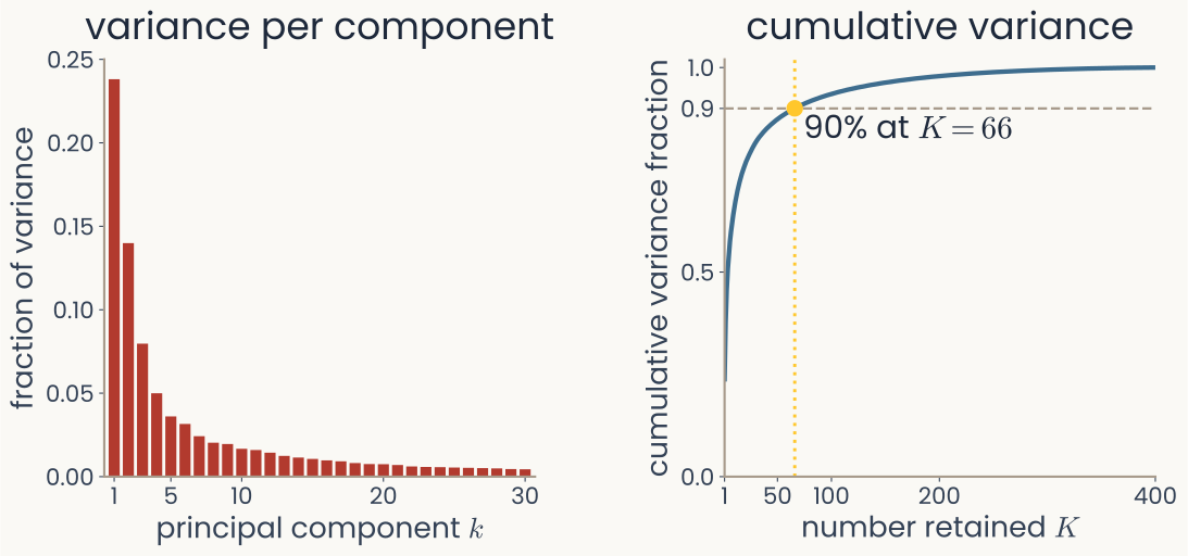
The scree plot from the PCA lecture for the 400 Olivetti faces: the variance fraction of the first 30 principal components falls steeply over the first few and then flattens, an elbow
Open full-size figure

From the PCA lecture: 400 Olivetti faces

Variance fraction $f_k = \lambda_k / \sum_j \lambda_j$ , largest first. An elbow = a natural place to stop

Slide 11

Mouse V1: variance fraction per component

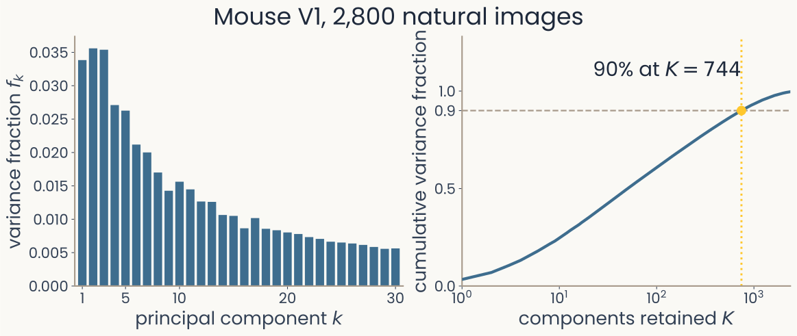
Two panels for mouse V1 responses to 2,800 natural images, averaged over seven sessions. Left: bars of the variance fraction of the first 30 principal components, falling slowly from about 0.035 to about 0.006 with no elbow. Right: cumulative variance fraction against components retained, on a log axis out to 2,366; a dashed line at 0.9 is crossed at K = 744
Open full-size figure

Computed from Stringer et al.'s data (7 sessions)

Two-photon imaging, ~10,000 neurons, each image shown twice. Cross-validated PCA: principal components from the first showing; each one's variance = how much the two showings co-vary along it, so trial noise cancels
No elbow: 90% of the variance needs 744 components

Slide 12

On log-log axes, a straight line

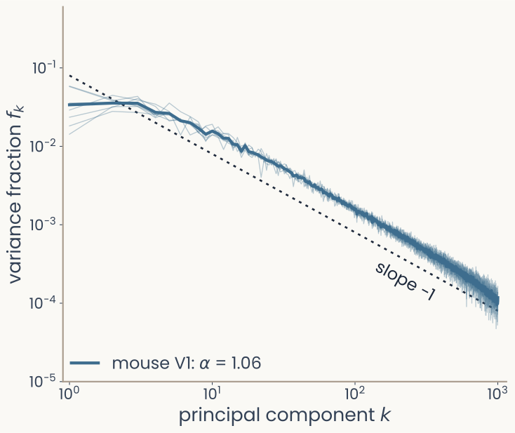
$Log-log plot of variance fraction against principal component k from 1 to 1,000 for mouse V1, seven thin lines for the recording sessions and one thick line for their mean, falling along a nearly straight line close to a dotted guide of slope minus 1; the legend gives alpha = 1.06$

Log-log plot of variance fraction against principal component k from 1 to 1,000 for mouse V1, seven thin lines for the recording sessions and one thick line for their mean, falling along a nearly straight line close to a dotted guide of slope minus 1; the legend gives alpha = 1.06

Computed from Stringer et al.'s data

Log-log axes: each tick is ×10, so a power law $f_k \propto k^{-\alpha}$ is a line of slope $-\alpha$
Mouse V1: straight over the measured range, $\alpha = 1.06$ (dotted: slope $-1$ )

Slide 13

No elbow: what it means

The log-log plot of variance fraction against principal component k for mouse V1 (2,800 images, alpha 1.06), a nearly straight line with no bend, beside a dotted guide of slope minus 1
Open full-size figure

Computed from Stringer et al.'s data

With an elbow, a few directions carry most of the variance: the embedding dimension is clear
Without one, the embedding dimension depends on the threshold (90%? 95%?)
V1 uses many dimensions, but unequally: each further component carries a little less. We want one number with no threshold
Why V1 has no elbow, and why it may matter for deep networks: see the appendix

Slide 14

One number: the participation ratio

The participation ratio of the eigenvalues $\lambda_k$ (variances along the principal components):

\mathrm{PR} = \frac{\left(\sum_j \lambda_j\right)^2}{\sum_j \lambda_j^2}, \qquad 1 \le \mathrm{PR} \le D

With the variance fractions $f_j$ : $\mathrm{PR} = 1/\sum_j f_j^2$ . Not to be confused with $f_k$ : one number per component; PR is one number for the whole spectrum
PR = 1 when one direction carries all the variance; PR = $D$ when all $D$ share it equally. No threshold; report $\mathrm{PR}/D$

The participation ratio counts how many directions the responses use: if k directions share the variance equally, PR = k. (minute paper)

Slide 15

Participation ratio, four populations

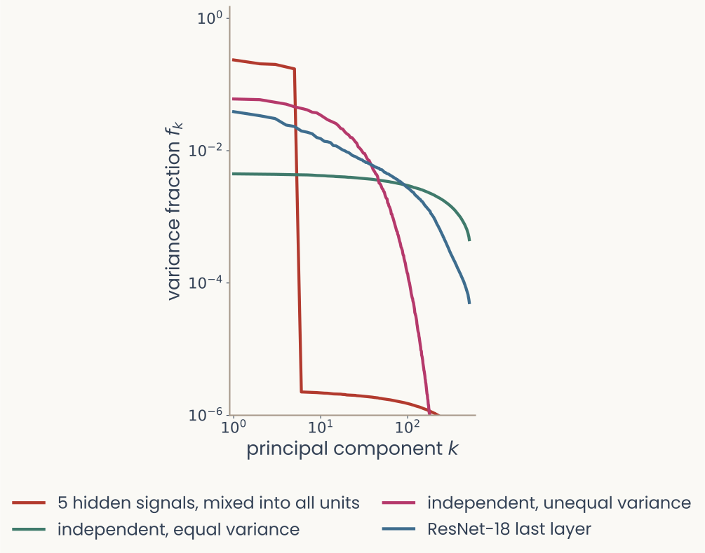
Log-log plot of variance fraction against principal component k for four populations of 512 units on 1,854 stimuli. 512 units that each mix the same five hidden signals: the first five components hold almost all the variance, PR about 5. Independent signals of equal variance: a nearly flat line, PR about 401. Independent signals of unequal variances: a line that falls steeply, PR about 32, although no unit is redundant. ResNet-18's last layer on 1,854 THINGS images: a line that falls steadily, PR 99
Open full-size figure

Simulated: 512 units, 1,854 stimuli, Gaussian signals + noise

5 hidden signals, each unit a different mix: units correlated, rank ≈ 5, PR ≈ 5
512 independent signals, one per unit, equal size: variance everywhere, PR ≈ 401
Same, but unequal sizes: the strongest few dominate, PR ≈ 32. ResNet-18: 99
PR counts how evenly the variance is spread, not how much information there is

Slide 16

Back to mouse V1

Computed from Stringer et al.'s data

~10,000 neurons recorded; 90% of the variance needs 744 components
Participation ratio: about 110 (75 to 145 per session)
One number for a spectrum with no elbow: many dimensions, used unequally

Slide 17

Scale matters: z-score or not

The eigenvalues are variances, so a unit measured on a large scale dominates them, and the participation ratio with them
z-score each unit (subtract its mean, divide by its standard deviation) when scales are arbitrary: fMRI voxels, calcium fluorescence. Keep the raw scale when sizes matter: spikes/s
z-scoring gives every unit variance 1: PR then counts patterns of co-activation, not loud units. Independent units of unequal size: PR 32 raw, 402 z-scored
ResNet-18 on THINGS: PR 99 raw, 107 z-scored. Report which you used

Slide 18

What can another neuron read from the responses?

Slide 19

What could another neuron use?

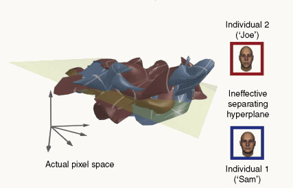
In pixel space the sheets of face images of two different people are interleaved, and a flat separating plane drawn through them fails to split them
Open full-size figure

Redrawn in the last lecture from DiCarlo & Cox (2007)

In pixels, two people's face images interleave: no flat (linear) plane separates them
"IT encodes animacy" is a claim about information another neuron could use
The simplest such neuron: a weighted sum and a threshold, a linear readout

DiCarlo & Cox Trends Cogn Sci 2007

Slide 21

A linear readout draws a hyperplane

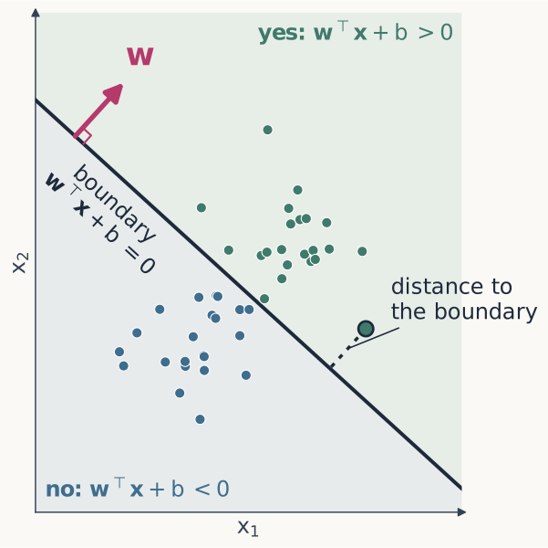
A 2-D plane with axes x1 and x2 holding two groups of dots, green "yes" points upper right and blue "no" points lower left. A fitted straight line runs between them and the two sides are lightly shaded. A magenta arrow labelled w starts on the line at a right angle and points into the green side. A dotted segment from a far point to the line is labelled distance

Toy data, computed

Response vector $\mathbf{x}$ , weights $\mathbf{w}$ , bias $b$ : the readout answers "yes" when $\mathbf{w}^{\top}\mathbf{x} + b > 0$
$\mathbf{w}^{\top}\mathbf{x} = w_1 x_1 + w_2 x_2$ , the dot product from the MDS lecture: one weight per unit
The boundary $\mathbf{w}^{\top}\mathbf{x} + b = 0$ : a line in 2-D, a plane in 3-D, a hyperplane in $D$ dimensions
$\mathbf{w}$ is perpendicular to it. Each point has a distance to the boundary

Slide 22

Monkey IT: reading animacy

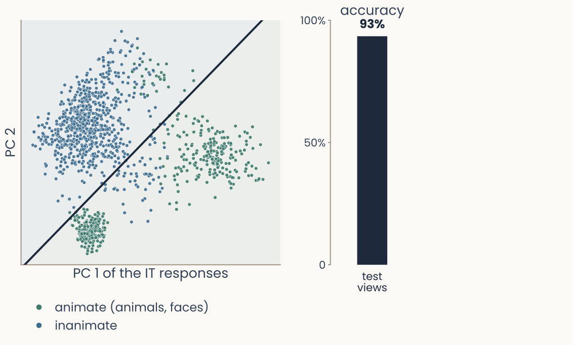
Monkey IT responses to the 1,224 Bao object images on their first two principal components. Green dots are animate images (animals and faces), blue dots inanimate ones. A straight tilted line fitted to the points separates most animate images from inanimate ones
Open full-size figure

Computed: monkey IT, 480 neurons, 2 principal components

Bao objects: 51 objects × 24 views, recorded in monkey IT, 480 neurons
Axes: IT's first two principal components. Green: animals and faces; blue: inanimate
Neither component alone separates them: the best boundary is tilted, a weighted sum of both
IT separates animate from inanimate objects (Kriegeskorte et al., 2008)

Bao et al. Nature 2020 · Kriegeskorte et al. Neuron 2008

Slide 25

Measuring with a readout

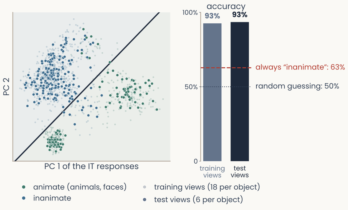
Monkey IT responses to the 1,224 Bao object images on their first two principal components. Faint dots are the 18 training views per object used to fit the line; solid dots are the 6 test views per object, held out, on which the line is scored
Open full-size figure

Computed: monkey IT, 480 neurons, 2 principal components

Result: the readout reads animacy correctly for 93% of the views. Is that a lot?
Baseline: guessing, 50%; always "inanimate", 63%: the majority-class baseline
Split: fit on 18 of each object's 24 views (training set); score on the other 6 (test set). Both 93%: the readout did not overfit

Bao et al. Nature 2020

Monkey IT responses to the 1,224 Bao object images on their first two principal components, animate views in green and inanimate in blue. Drag a straight line with two handles; meters give the share of training views it classifies correctly and, once revealed, the share of test views, against the majority-class baseline. A button fits a readout — open interactive version

Slide 26

Draw the boundary yourself

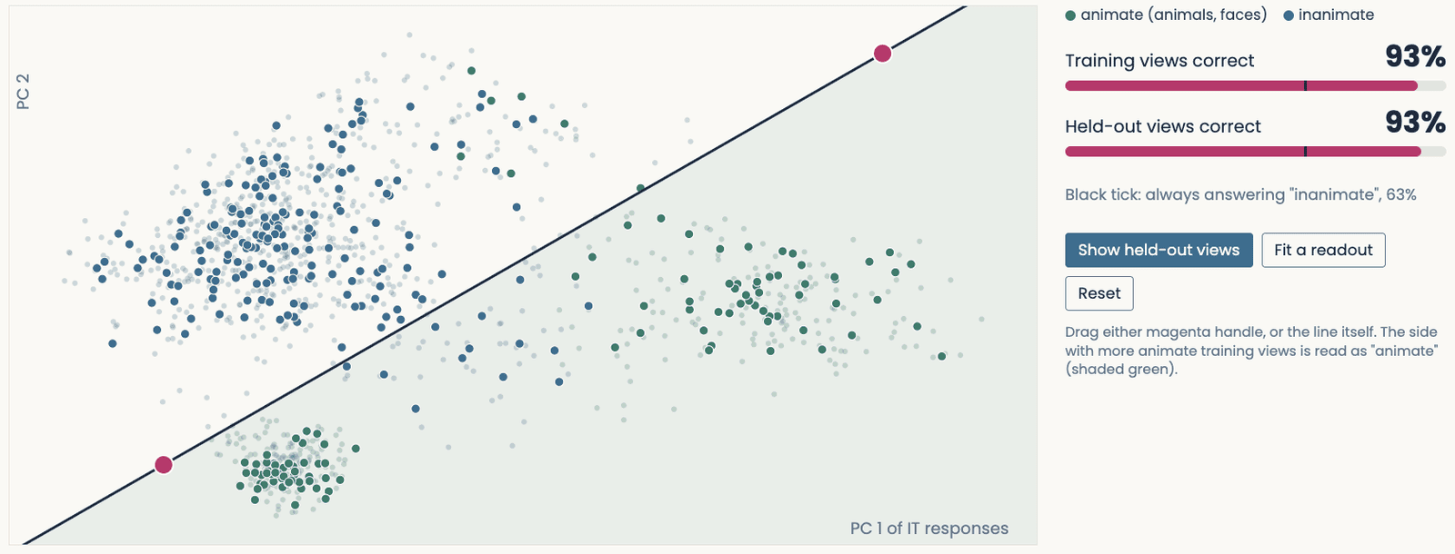
The readout demo with the fitted line: the share of training views and of test views classified correctly, against the majority-class baseline
Open full-size figure

Each point has a distance to the boundary; points near it flip when the boundary moves

Slide 29

Linearly separable, or not

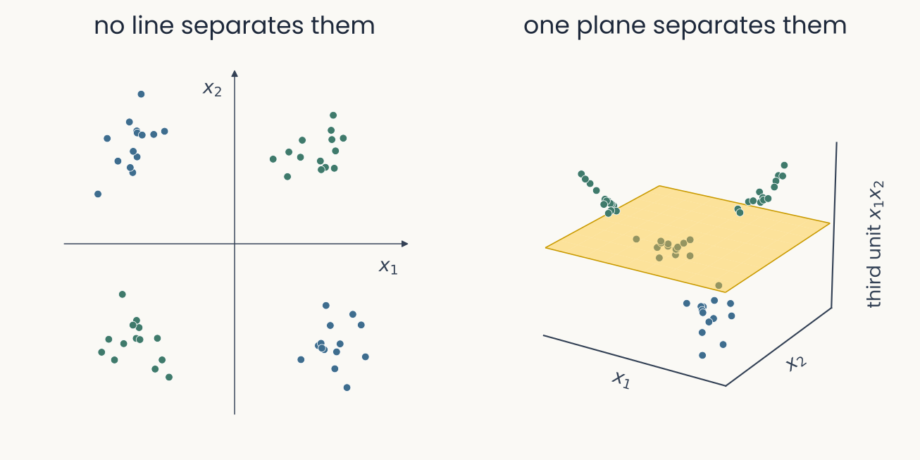
Toy data, two panels side by side at the same size. Left, the XOR clusters in the plane of x1 and x2. Right, the same clusters lifted by a third unit x1 times x2: the green clusters rise above a translucent plane and the blue ones drop below it, so one plane separates them
Open full-size figure

Toy data, computed: inputs coded −1 and +1

Two classes are linearly separable when one hyperplane puts them on opposite sides
XOR: green when both inputs have the same sign. No boundary works: 75% at best
A third unit $x_1 x_2$ lifts the points into 3-D: one plane separates them

Slide 30

Minute paper

Submit on Canvas → Minute papers → Minute Paper 6 (access code read out in class).

Write three brief points in your own words:

What does the participation ratio measure?
If k directions share the variance equally, what is its value?
Something you do not yet understand, or a question still open
Another idea you found interesting, and why it matters for brains, behavior or AI

Credit for a thoughtful attempt, not for being correct.

Slide 32

Appendix: derivations and extra examples

Material not covered in class, for reference

Slide 33

Going further: what does the power law mean?

Slide 34

Monkey V1 falls the same way

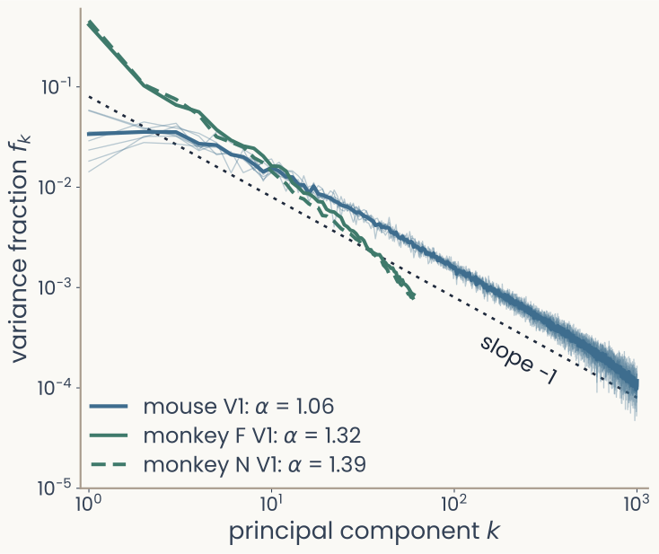
The same log-log plot with monkey V1 added: two green lines, one per monkey, for principal components 1 to 60, starting higher and falling a little more steeply than the mouse line, with alpha 1.32 and 1.39
Open full-size figure

Computed from Stringer et al.'s and Papale et al.'s data

Log-log axes: each tick is ×10, so a power law $f_k \propto k^{-\alpha}$ is a line of slope $-\alpha$
Mouse V1: straight over the measured range, $\alpha = 1.06$ (dotted: slope $-1$ )
Monkey V1: electrode arrays; 100 THINGS images (photos of everyday objects). A little steeper, $\alpha = 1.32$ and $1.39$

Stringer et al. Nature 2019 · Papale et al. Neuron 2025

Slide 35

Pixels fall the same way

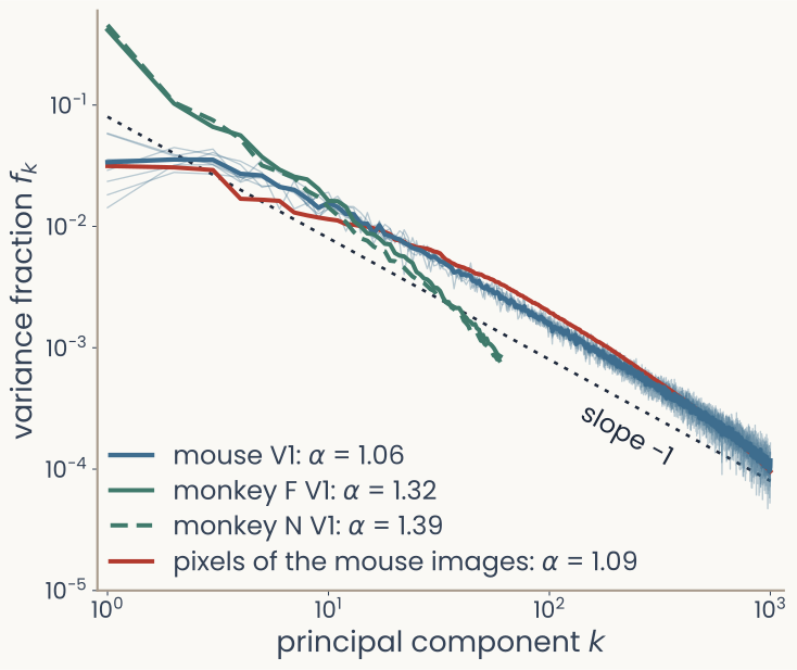
The same log-log plot with a red line added for the pixels of the 2,800 images the mice saw: it falls almost exactly on top of the mouse V1 line, alpha 1.09
Open full-size figure

Computed from Stringer et al.'s and Papale et al.'s data

Log-log axes: each tick is ×10, so a power law $f_k \propto k^{-\alpha}$ is a line of slope $-\alpha$
Mouse V1: straight over the measured range, $\alpha = 1.06$ (dotted: slope $-1$ )
Monkey V1, electrode arrays, 100 THINGS images: a little steeper, $\alpha = 1.32$ and $1.39$
Pixels of the 2,800 images: $\alpha = 1.09$ , the same slope. Is V1 just copying the images?

Stringer et al. Nature 2019 · Papale et al. Neuron 2025

Slide 36

Neurons are not pixels

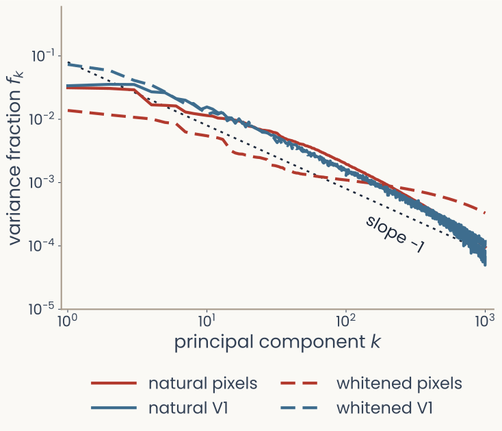
$Log-log plot of variance fraction against principal component k for natural and whitened images. For natural images the pixel spectrum, alpha 1.09, and the mouse V1 spectrum, alpha 1.06, lie almost on top of each other. For whitened images the pixel spectrum is much flatter, alpha 0.41, while the mouse V1 spectrum still follows the dotted line of slope minus 1, alpha 1.09$

Log-log plot of variance fraction against principal component k for natural and whitened images. For natural images the pixel spectrum, alpha 1.09, and the mouse V1 spectrum, alpha 1.06, lie almost on top of each other. For whitened images the pixel spectrum is much flatter, alpha 0.41, while the mouse V1 spectrum still follows the dotted line of slope minus 1, alpha 1.09

Stringer et al.'s data: 7 natural, 4 whitened sessions

Whitened images: all scales, equal contrast
Their pixels flatten: $\alpha$ from 1.09 to 0.41. Mouse V1 does not: 1.06 to 1.09
V1's power law is not inherited from the images
It is a property of how V1 encodes images (why a slope near 1 matters: two slides on)

Slide 37

A power law across species and methods

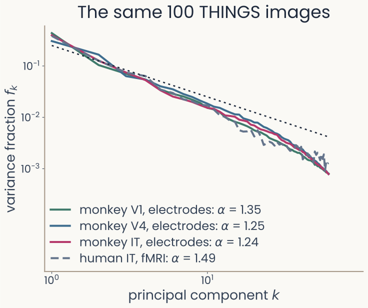
Log-log plot of variance fraction against principal component k from 1 to 60 for the same 100 THINGS images in monkey V1, V4 and IT (electrodes) and human visual cortex (fMRI), all with the same cross-validated estimator. All four fall along nearly parallel straight lines, with alpha 1.35, 1.25, 1.24 and 1.49
Open full-size figure

Computed here: one estimator, 100 THINGS images

Variance falls as a power law: mouse V1; monkey V1, V4, IT; human cortex
Calcium imaging, electrodes, fMRI: same shape; the exponent depends on the estimator
Shepard's law of generalization (MDS lecture) was such a law for behavior
A candidate law of neural coding

Gauthaman et al. PLoS Comput Biol 2025 · Shepard Science 1987

Slide 38

Why a slope near 1? A smooth code

$Log-log plot of variance fraction against principal component k from 1 to 1,000 for mouse V1 responses to 2,800 natural images: seven thin lines for the recording sessions and one thick line for their mean, falling along a nearly straight line close to a dotted guide of slope minus 1; alpha 1.06$

Log-log plot of variance fraction against principal component k from 1 to 1,000 for mouse V1 responses to 2,800 natural images: seven thin lines for the recording sessions and one thick line for their mean, falling along a nearly straight line close to a dotted guide of slope minus 1; alpha 1.06

Computed from Stringer et al.'s data

Smooth code: similar images give similar responses, as small changes should
Slower than $1/k$ : fine directions dominate; near-identical images land far apart
Stringer et al.'s theory: a slope near $-1$ is about the flattest a smooth code allows. V1 uses as many dimensions as smoothness permits
Why that matters: networks are not smooth

Slide 39

Deep networks are fooled by invisible changes

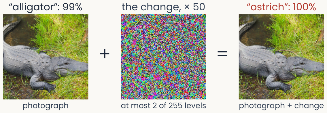
Three images in a row. Left, a public-domain photograph of an alligator lying on grass, which ImageNet-trained ResNet-18 labels alligator with 99 percent probability. Middle, the change added to it, magnified 50 times: colored noise; no pixel moves by more than 2 of 255 intensity levels. Right, the photograph plus the change, which looks identical to the original, labeled ostrich with 100 percent probability

Computed here: ResNet-18 trained on ImageNet, a public-domain THINGS photograph

Adversarial attack: a change of ≤ 2 of 255 levels per pixel flips the network's answer; we still see the same alligator in both photographs
It matters for cars, medical imaging and face recognition, and no defense removes the problem

Szegedy et al. ICLR 2014 · Madry et al. ICLR 2018

Slide 40

Could a V1-like spectrum make networks robust?

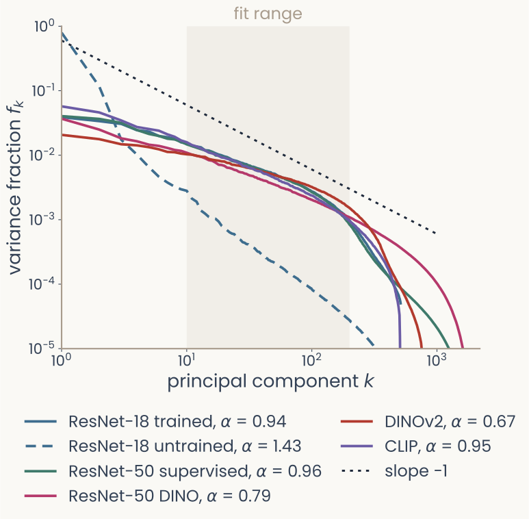
Log-log plot of the variance fraction of each principal component against its number k, for six networks' last layers on 1,854 THINGS images, with a dotted line of slope minus 1. Five trained networks fall more gently than the dotted line, with exponents between 0.67 and 0.96; the untrained ResNet-18, dashed, falls more steeply, exponent 1.43
Open full-size figure

Six networks, computed here: trained ones are flatter than V1 (0.67–0.96 vs 1.06)
Kong et al. (2022): networks trained to resist attacks have steeper, more V1-like spectra
Nassar et al. (2020): a training penalty pulls a layer's spectrum toward $1/k$ : harder to fool
Open: is robustness why V1 has a power law?

Kong et al. PLoS Comput Biol 2022 · Nassar et al. NeurIPS 2020

Slide 41

Effective dimensionality from an eigenspectrum

import numpy as np
# X: (N stimuli, D units) response matrix -- neurons, voxels or model units
Xc = X - X.mean(axis=0, keepdims=True)          # center: PCA needs it (the PCA lecture)

C = Xc.T @ Xc / (Xc.shape[0] - 1)               # the D x D covariance matrix
lam = np.sort(np.linalg.eigvalsh(C))[::-1]      # its eigenvalues, largest first
lam = lam[lam > 0]

pr = lam.sum()**2 / (lam**2).sum()              # participation ratio, 1 <= PR <= D
print(f"ambient D = {X.shape[1]},  effective dimensionality = {pr:.1f}")

f = lam / lam.sum()                             # variance fraction f_k of component k
k = np.arange(1, len(f) + 1)
alpha = -np.polyfit(np.log(k[10:500]), np.log(f[10:500]), 1)[0]
print(f"variance fraction decays as k^-{alpha:.2f}")

Elhage et al. Transformer Circuits Thread 2022

Slide 42

More features than units

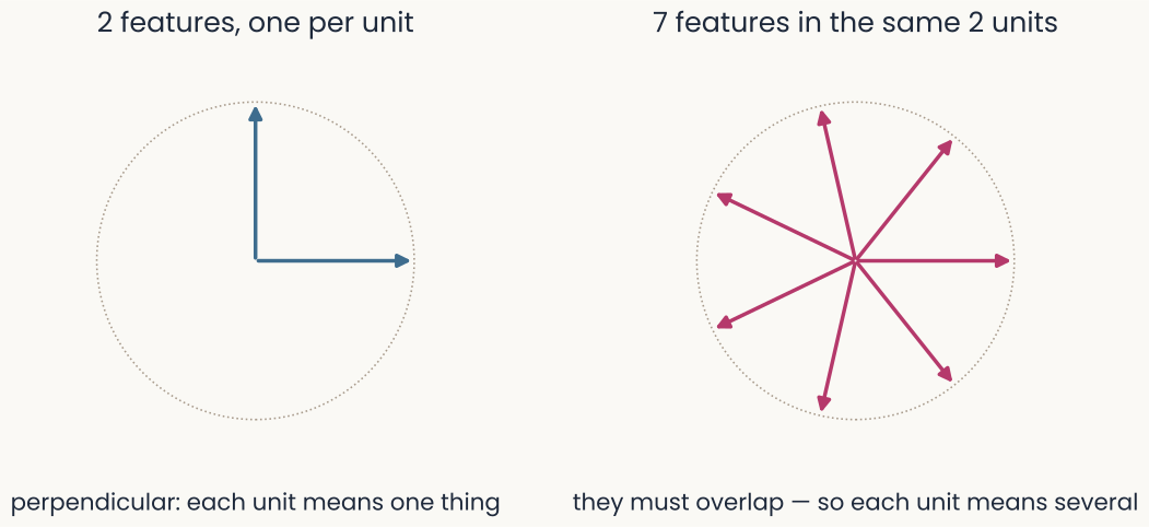
Two circles of directions: two perpendicular feature directions where each unit means one thing, versus seven directions packed into the same plane, forced to overlap
Open full-size figure

$D$ perpendicular directions hold at most $D$ features. Nearly perpendicular directions, plentiful in high dimensions, hold far more, and each unit sits on several
A population can code more features than it has units: no unit stands for one thing