Hidden layers & backpropagation

Reader-friendly version of the 39 lecture slides: the lecture content in normal flow, with figure descriptions and data tables where the figure carries data. Open the presentation.

Slide 1

CPSY 1291 Computational Methods for Mind, Brain & Behavior

Lecture 9 · Theme 2: Learning representations: from neurons to deep networks

Hidden layers & backpropagation

Tuesday, October 13 · Fall 2026

Return to contents

Slide 2

Last lecture: one neuron that learns

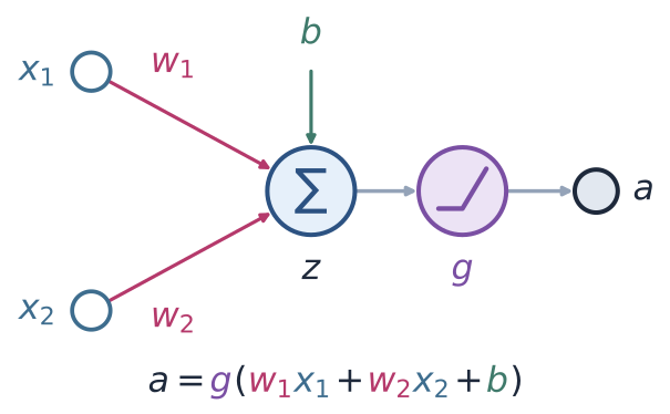
A model neuron with two inputs, x1 and x2, with weights w1 and w2, summed with a bias b into z, passed through the nonlinearity g, giving the output a = g(w1 x1 + w2 x2 + b)
Open full-size figure

Perceptron: $\hat y = \mathrm{sign}(z)$ , labels $\pm 1$
Delta rule: $\hat y = z$ , squared error
Logistic regression: $\hat y = \sigma(z)$ , cross-entropy

The model neuron: a weighted sum $z = \textcolor{#B5396B}{\mathbf{w}}^\top\textcolor{#3E6D8E}{\mathbf{x}} + \textcolor{#3F7A6B}{b}$ , then a nonlinearity $a = \textcolor{#7A4FA3}{g}(z)$ . Its weights set one decision boundary
Learning: the loss $\ell$ measures the gap between the output $\hat y = a$ and the target $y$ ; the weights move against its gradient
All three rules of last lecture share one update: learning rate × error × input

\Delta \textcolor{#B5396B}{\mathbf{w}} = \eta\,(y-\hat y)\,\textcolor{#3E6D8E}{\mathbf{x}}

Return to contents

Slide 3

Learning the weights: start anywhere, walk downhill

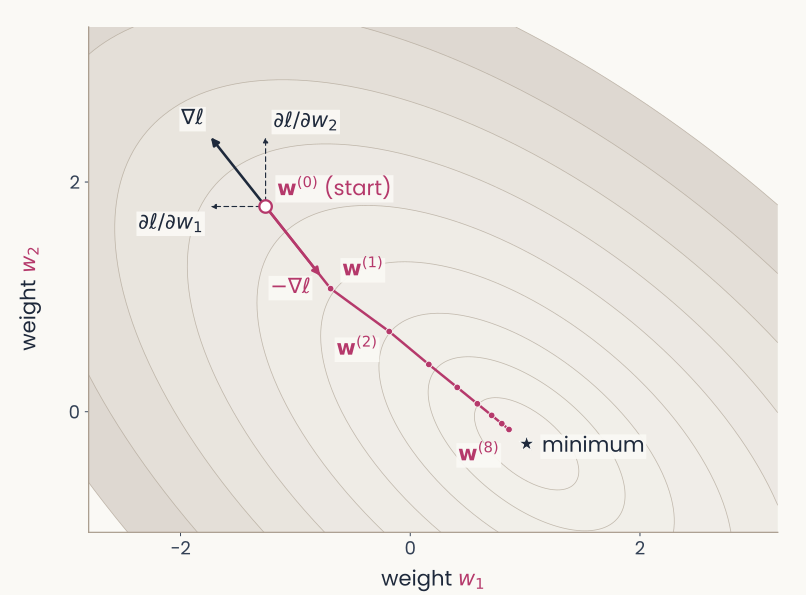
Contours of the loss over the two weights w1 and w2, with the minimum marked by a star. At the start w(0), at the upper left, a dark arrow shows the gradient pointing uphill, with dashed arrows for its two components, the partial derivatives with respect to w1 and w2. A magenta arrow labelled minus the gradient points the other way, to w(1); eight dots w(0) to w(8) step down toward the minimum

Open full-size figure

Each pair $(w_1, w_2)$ has a loss $\ell$ : the squared error $\tfrac12(y-\hat y)^2$ , averaged over a small training set; contours join equal losses
Start at small random weights $\textcolor{#B5396B}{\mathbf{w}}^{(0)}$ . The gradient $\nabla\ell = (\partial\ell/\partial w_1,\ \partial\ell/\partial w_2)$ points uphill, toward higher loss
Each step is a weight update against the gradient; the learning rate $\eta$ sets its size

\textcolor{#B5396B}{\mathbf{w}}^{(t+1)} = \textcolor{#B5396B}{\mathbf{w}}^{(t)} - \eta\,\nabla\ell

For this neuron the loss is convex, a bowl with a single minimum. From any start, small enough steps reach the bottom

Return to contents

Slide 4

You never see the whole landscape

The contour map was drawn by computing $\ell$ for every pair $(w_1, w_2)$ on a grid: easy with only 2 weights
With 100 weights and only 10 values tried per weight, the grid has $10^{100}$ points. Real networks have millions of weights: the map can never be drawn
Gradient descent never needs the map. At the current weights it computes the gradient: for each weight, which way to move to lower $\ell$ , and how strongly
Why that is cheap: the gradient is a formula, worked out once with calculus (next slides). Its cost grows in proportion to the number of weights, not exponentially as the grid does
Each small step lowers the loss. A step computed from one example, or from a small batch of examples (minibatches, next lecture), lowers it on average

Return to contents

Slide 5

The chain rule, one link at a time

The weights change the loss only through a chain: $\textcolor{#B5396B}{\mathbf{w}} \;\to\; z = \textcolor{#B5396B}{\mathbf{w}}^\top \textcolor{#3E6D8E}{\mathbf{x}} + \textcolor{#3F7A6B}{b} \;\to\; \hat y = \textcolor{#7A4FA3}{g}(z) \;\to\; \ell$
Chain rule of calculus: if $\ell = f(u)$ and $u = h(w)$ , then $\dfrac{d\ell}{dw} = \dfrac{d\ell}{du}\,\dfrac{du}{dw}$ . A longer chain multiplies one slope per link. This gives the gradient of the loss with respect to each weight

\frac{\partial\ell}{\partial \textcolor{#B5396B}{\mathbf{w}}}=\frac{\partial\ell}{\partial\hat y}\;\frac{\partial\hat y}{\partial z}\;\frac{\partial z}{\partial \textcolor{#B5396B}{\mathbf{w}}}

Link $\hat y \to \ell$ : $\;\partial\ell/\partial\hat y$ , set by the loss
Link $z \to \hat y$ : $\;\partial\hat y/\partial z = \textcolor{#7A4FA3}{g}'(z)$ , the slope of the nonlinearity
Link $\textcolor{#B5396B}{\mathbf{w}} \to z$ : $\;\partial z/\partial \textcolor{#B5396B}{\mathbf{w}} = \textcolor{#3E6D8E}{\mathbf{x}}$ , because $z = w_1x_1 + w_2x_2 + b$
Multiply the three slopes and you have the gradient

Return to contents

Slide 6

The three links, worked out: delta rule

Output $\hat y = z$ (no nonlinearity), loss $\ell = \tfrac12(y-\hat y)^2$

\frac{\partial\ell}{\partial\hat y} = \tfrac12\cdot 2\,(y-\hat y)\cdot(-1) = -(y-\hat y)

\frac{\partial\hat y}{\partial z} = 1 \qquad\qquad \frac{\partial z}{\partial \textcolor{#B5396B}{\mathbf{w}}} = \textcolor{#3E6D8E}{\mathbf{x}}

\frac{\partial\ell}{\partial \textcolor{#B5396B}{\mathbf{w}}} = -(y-\hat y)\cdot 1\cdot \textcolor{#3E6D8E}{\mathbf{x}} = -(y-\hat y)\,\textcolor{#3E6D8E}{\mathbf{x}}

The error $\delta = y-\hat y$ gives the rule its name. Step against the gradient: $\Delta \textcolor{#B5396B}{\mathbf{w}} = \eta\,\delta\,\textcolor{#3E6D8E}{\mathbf{x}}$ , the delta rule
Backpropagation, later, writes the error with the opposite sign: $\delta = \partial\ell/\partial z = \hat y - y$

Return to contents

Slide 7

The three links, worked out: logistic regression

Output $\hat y = \sigma(z) = \dfrac{1}{1+e^{-z}}$ , loss $\ell = -\big[\,y\log\hat y + (1-y)\log(1-\hat y)\,\big]$

\frac{\partial\ell}{\partial\hat y} = -\frac{y}{\hat y}+\frac{1-y}{1-\hat y} = \frac{-y(1-\hat y)+(1-y)\,\hat y}{\hat y(1-\hat y)} = -\frac{y-\hat y}{\hat y(1-\hat y)}

\frac{\partial\hat y}{\partial z} = \sigma(z)\big(1-\sigma(z)\big) = \hat y(1-\hat y) \qquad\qquad \frac{\partial z}{\partial \textcolor{#B5396B}{\mathbf{w}}} = \textcolor{#3E6D8E}{\mathbf{x}}

\frac{\partial\ell}{\partial \textcolor{#B5396B}{\mathbf{w}}} = -\frac{y-\hat y}{\hat y(1-\hat y)}\cdot\hat y(1-\hat y)\cdot \textcolor{#3E6D8E}{\mathbf{x}} = -(y-\hat y)\,\textcolor{#3E6D8E}{\mathbf{x}}

The sigmoid's slope cancels the loss's denominator: the same form as the delta rule

Return to contents

Slide 8

The perceptron is gradient descent after all

Last lecture: Rosenblatt's rule was a heuristic. On each mistake, add $\eta\,y\,\textcolor{#3E6D8E}{\mathbf{x}}$ (labels $y=\pm1$ ). Its threshold output has no slope, so the chain rule cannot derive it
Now treat the output as linear, $\hat y = z$ , and score it with $\ell = \max(0,\,-y\,z)$ : 0 when the example is on the correct side, growing with how far a mistake is on the wrong side
The gradient is $-y\,\textcolor{#3E6D8E}{\mathbf{x}}$ on a mistake, 0 otherwise. Stepping against it gives exactly Rosenblatt's rule
The heuristic is gradient descent on this loss, the hinge loss with a margin of 0

Return to contents

Slide 9

Why more than one layer?

Return to contents

Slide 10

One line fails on XOR; simpler rules do not

XOR (first panel below): one neuron, one line, at best 3 of the 4 points right
But XOR is built from simpler rules, each one perceptron with one line (other panels):

x_1 \,\text{XOR}\, x_2 = (x_1 \lor x_2) \land \lnot(x_1 \land x_2)

Stack them: OR and NOT-AND in a first layer, a neuron combining them in a second

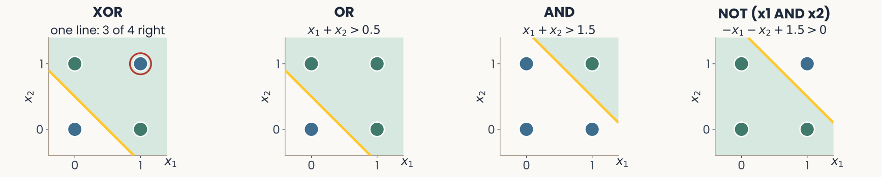
Four small panels. XOR: the four inputs with the best single line, 3 of 4 right, the wrong point (1,1) circled. OR: the four inputs, with (0,1), (1,0) and (1,1) green and (0,0) blue, separated by the gold line x1 + x2 = 0.5. AND: only (1,1) green, separated by the line x1 + x2 = 1.5. NOT (x1 AND x2): the four inputs, green except (1,1) in blue, separated by the gold line x1 + x2 = 1.5, shaded below it
Open full-size figure

Return to contents

Slide 11

Stack them: two hidden units and one output

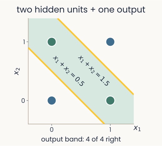
The four XOR points, blue at (0,0) and (1,1), green at (0,1) and (1,0). Two hidden units, then one output: two gold lines, x1 + x2 = 0.5 and x1 + x2 = 1.5, bound a band that is the output's green region, and all 4 points are right
Open full-size figure

Two hidden units, one like OR and one like AND; the output adds OR and subtracts AND (the NOT), so it fires in the band between their lines: all 4 right
A multilayer perceptron (MLP) stacks layers: each layer's outputs are the next layer's inputs, and every unit takes a weighted sum, then a nonlinearity. Stacked neurons draw boundaries that one line cannot

Return to contents

Slide 12

The hidden layer re-represents the input

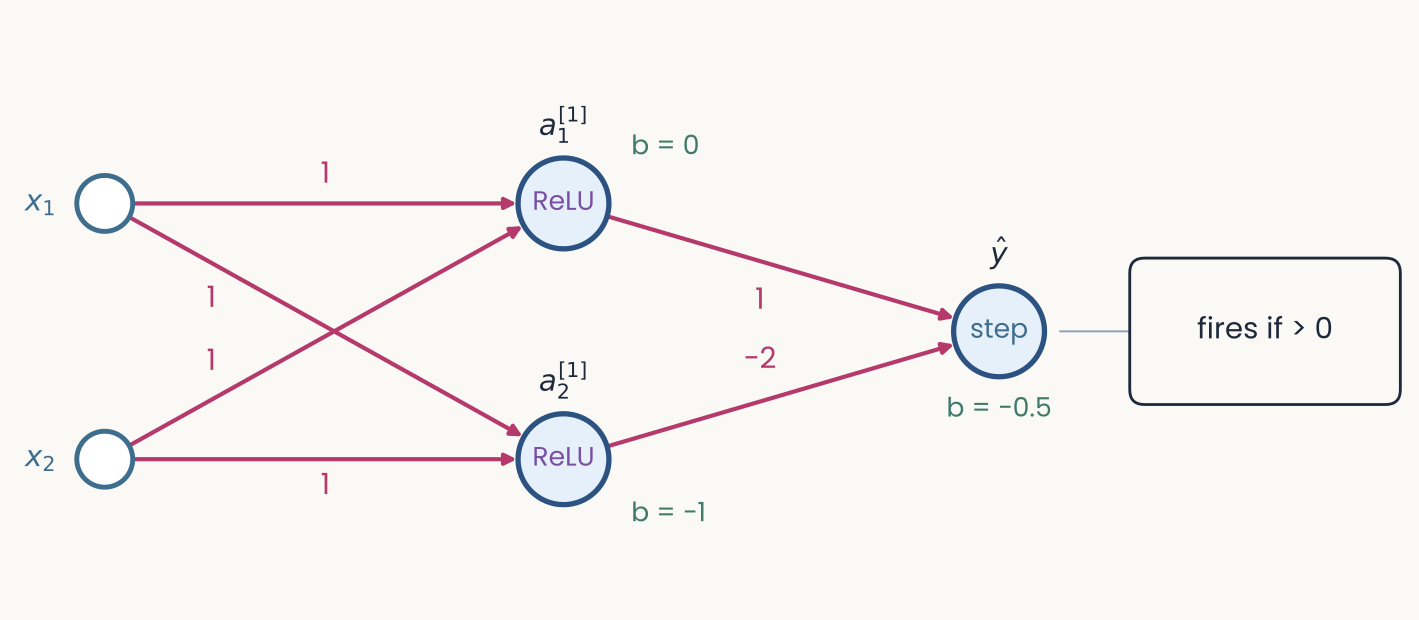
The XOR network of the previous slide: inputs x1 and x2, weights of 1 into both ReLU hidden units, biases 0 and minus 1, output weights 1 and minus 2, output is a step unit with bias minus 0.5
Open full-size figure

$a^{[l]}_j$ : output of unit $j$ in layer $l$ (layer 1 is hidden). With ReLUs, unit 1 acts like OR, unit 2 like AND
In the plane of $a^{[1]}_1, a^{[1]}_2$ , (0,1) and (1,0) land on one point: one line separates the classes
The hidden layer turns XOR into a linearly separable problem for the readout

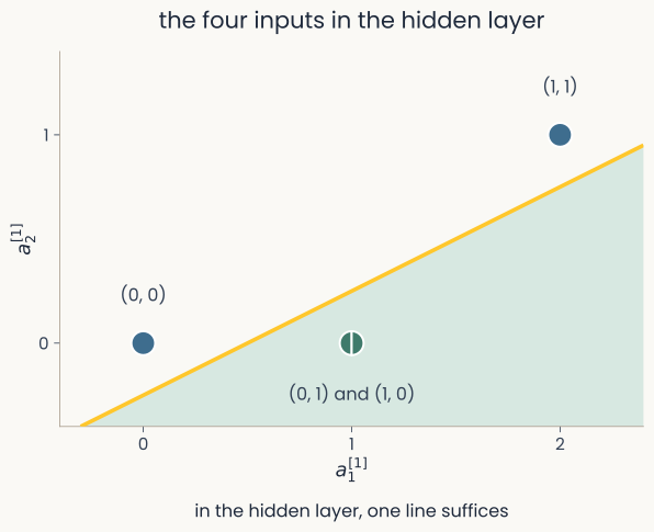
The four XOR inputs in hidden-unit coordinates a1 and a2 of layer 1: blue (0,0) at the origin, green (0,1) and (1,0) together at (1,0), blue (1,1) at (2,1). One solid gold line separates the green point, on the shaded side, from the two blue points. The caption reads: in the hidden layer, one line suffices
Open full-size figure

Return to contents

Slide 13

Why the ReLU matters: linear layers collapse into one

Remove the ReLUs from the XOR network: $a^{[1]}_1 = x_1 + x_2$ and $a^{[1]}_2 = x_1 + x_2 - 1$
The output's sum becomes $a^{[1]}_1 - 2a^{[1]}_2 - 0.5 = -(x_1 + x_2) + 1.5$ : one weighted sum of the inputs, so one line again, and XOR is lost
A weighted sum of weighted sums is a weighted sum. Without a nonlinearity, stacking adds nothing
With the ReLU, unit 2 stays at 0 until $x_1 + x_2 > 1$ . That bend is what turns two lines into a band

Return to contents

Slide 14

With hidden layers, the landscape is no longer a bowl

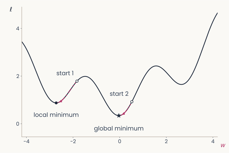
A loss curve over one weight w with three valleys of different depths. Two starting points chosen at random; gradient descent from each follows the curve downhill to a different valley: one reaches the deepest valley, marked global minimum, the other stops in a shallower valley, marked local minimum
Open full-size figure

Once a network has hidden layers, the loss is not convex: it has many valleys, local minima
Gradient descent still goes down from wherever it starts. Different starts can end in different minima; none is guaranteed best
In practice, large networks usually reach a minimum that works well. That is an observation, not a guarantee

Return to contents

Slide 15

How can a hidden unit learn when nothing tells it what to output?

Return to contents

Slide 16

Backpropagation: a long and disputed history

1958: Rosenblatt's perceptron learns its weights from examples, but only one layer of them
1969: Minsky & Papert show that a perceptron cannot compute XOR. No widely known method trains hidden layers, and interest in neural networks fades
1970–1974: Linnainmaa, studying rounding errors in computer programs, computes all the derivatives of a long calculation in one backward sweep. Werbos: general models in 1974, neural networks in 1982
1986: Rumelhart, Hinton & Williams show that hidden units trained this way learn useful internal representations. Their Nature paper made backprop the standard method
Who deserves the credit is still argued. Hinton's 2024 Nobel Prize in Physics, shared with Hopfield, cited a different kind of network, the Boltzmann machine, not backprop. His 2018 Turing Award, shared with Bengio and LeCun, was for deep learning as a whole

Rosenblatt Psychol Rev 1958 · Rumelhart, Hinton & Williams Nature 1986 · NobelPrize.org Physics 2024 · ACM Turing Award 2018

Return to contents

Slide 17

Notation for a network with layers

Layers are numbered: the input is layer 0, $\mathbf{a}^{[0]}=\mathbf{x}$ ; the output is the last layer, $L$ , so $\hat y = a^{[L]}$ ( $L$ = number of layers)
Unit $j$ of layer $l$ : weighted sum $z^{[l]}_j$ , output $a^{[l]}_j = g\big(z^{[l]}_j\big)$
$\textcolor{#B5396B}{w}^{[l]}_{jk}$ : one weight (a number), into unit $j$ of layer $l$ from unit $k$ of the layer below: $z^{[l]}_j = \sum_k \textcolor{#B5396B}{w}^{[l]}_{jk}\,a^{[l-1]}_k + b^{[l]}_j$ , with bias $b^{[l]}_j$ . Layer $l$ 's weights form the matrix $\textcolor{#B5396B}{\mathbf{W}}^{[l]}$

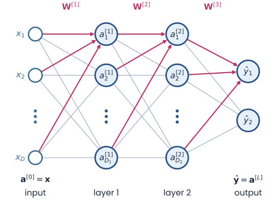
A fully connected network drawn left to right: inputs x1 to xD (a superscript 0 equals x), hidden layer 1 with units a superscript 1, hidden layer 2 with units a superscript 2, and an output layer y-hat. Every unit connects to every unit of the next layer; the weight matrices W superscript 1, 2 and 3 label the gaps
Open full-size figure

Return to contents

Slide 18

Nudge a hidden unit and follow the effect

How does the loss change if hidden unit $j$ 's weighted sum $z^{[1]}_j$ grows by a small amount $\varepsilon$ ?

Nudge a hidden unit and follow the effect — table
	follows the chain	in math
1	its output $a^{[1]}_j = g(z^{[1]}_j)$ moves by its slope × $\varepsilon$	$g'(z^{[1]}_j)\,\varepsilon$
2	the output unit's sum $z^{[2]}$ moves by the connecting weight × that	$\textcolor{#B5396B}{w}^{[2]}_j\,g'(z^{[1]}_j)\,\varepsilon$
3	the loss moves by the output's error × that, as in logistic regression	$(\hat y - y)\,\textcolor{#B5396B}{w}^{[2]}_j\,g'(z^{[1]}_j)\,\varepsilon$

The loss change per unit nudge is the hidden unit's error: $\delta^{[1]}_j = (\hat y - y)\,\textcolor{#B5396B}{w}^{[2]}_j\,g'(z^{[1]}_j)$ , the output error sent back through the weight
It plays the role $\hat y - y$ plays for the output. Each weight into the hidden unit changes by error × input: $\partial\ell/\partial \textcolor{#B5396B}{w}^{[1]}_{jk} = \delta^{[1]}_j\,x_k$

Return to contents

Slide 19

Backpropagation: the recipe, for any network

Forward: run the input through and keep every weighted sum $z$ and output $a$
Output error: the output has a target, so its error is $\;\delta_{\text{out}} = \hat y - y$
Backward: each hidden unit's error = the errors of the units it feeds, each × the weight to them, all × its own slope: $\;\delta_j = g'(z_j)\,\sum_k \textcolor{#B5396B}{w}_{kj}\,\delta_k$
Gradients: each weight's gradient = error of the unit it enters × its input: $\partial\ell/\partial \textcolor{#B5396B}{w} = \delta \times \text{input}$

Why backward: step 3 for one layer needs the errors of the layer above. Start at the output and work back, layer by layer

Return to contents

Slide 20

Where the recipe comes from: the chain rule

A unit's error is the slope of the loss with respect to its weighted sum: $\;\delta = \partial\ell/\partial z$
Output unit: chain through $\hat y$ (logistic regression, earlier):

\delta_{\text{out}} = \frac{\partial\ell}{\partial\hat y}\,\frac{\partial\hat y}{\partial z_{\text{out}}} = \hat y - y

Hidden unit $j$ : $z_j$ changes the loss through every unit $k$ it feeds, so the chains add up:

\delta_j = \frac{\partial\ell}{\partial z_j} = \sum_k \underbrace{\frac{\partial\ell}{\partial z_k}}_{\textstyle\delta_k}\;\underbrace{\frac{\partial z_k}{\partial a_j}}_{\textstyle \textcolor{#B5396B}{w}_{kj}}\;\underbrace{\frac{\partial a_j}{\partial z_j}}_{\textstyle g'(z_j)} \qquad\qquad \frac{\partial\ell}{\partial \textcolor{#B5396B}{w}_{jk}} = \underbrace{\frac{\partial\ell}{\partial z_j}}_{\textstyle\delta_j}\;\underbrace{\frac{\partial z_j}{\partial \textcolor{#B5396B}{w}_{jk}}}_{\textstyle a_k}

Each formula of the recipe is the chain rule, with the slopes we already know

Return to contents

Slide 21

Back to XOR: learn the weights from random ones

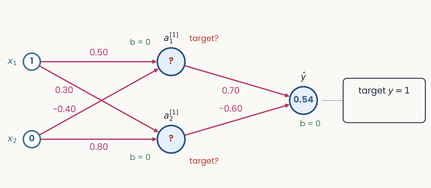
A 2-2-1 network drawn left to right. Inputs x1 = 1 and x2 = 0; six magenta weights; two hidden units marked with red question marks and the words target?; an output unit at 0.54; a box on the right reading target y = 1
Open full-size figure

Above: the XOR network before training, with small random weights instead of the hand-set ones. Hidden units ReLU. Output: a sigmoid with the cross-entropy, so $\hat y$ is a probability (a linear output with squared error would also train; threshold only to read the class)
Input (1, 0), target 1: the output is $\hat y = 0.54$ . Four steps compute every gradient

Return to contents

Slide 23

Step 1: the forward pass

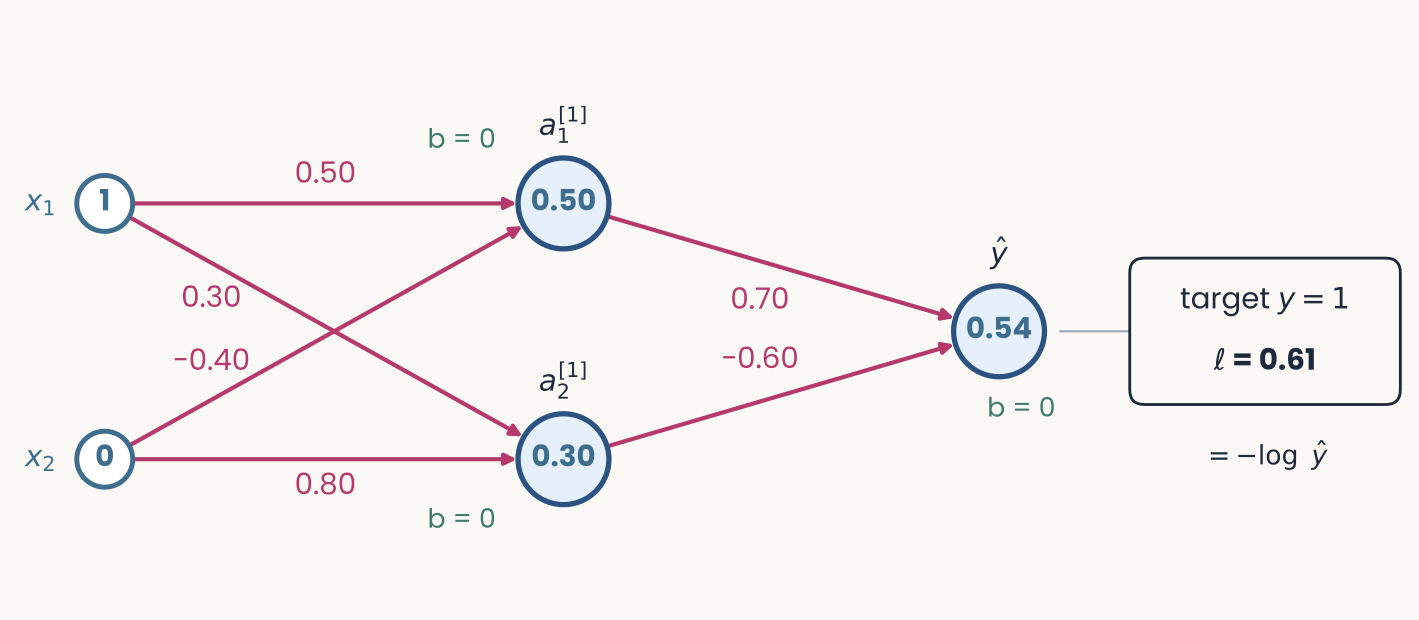
The same network after the forward pass. The box on the right now reads target y = 1, loss 0.61, and underneath, equals minus log y hat
Open full-size figure

Hidden: $z^{[1]}_1 = 0.50\cdot 1 - 0.40\cdot 0 + 0 = 0.50$ , $\;z^{[1]}_2 = 0.30\cdot 1 + 0.80\cdot 0 + 0 = 0.30$
Output: $z^{[2]} = 0.70\cdot 0.50 - 0.60\cdot 0.30 + 0 = 0.17$ , $\;\hat y = \sigma(0.17) = 0.54$
Loss: $\ell = -\big[y\log\hat y + (1-y)\log(1-\hat y)\big] = -\big[\log 0.542 + 0\big] = 0.61$

Return to contents

Slide 24

Step 2: the error at the output

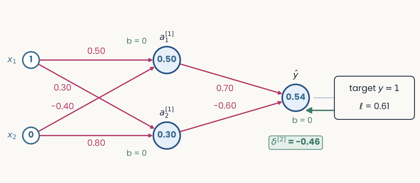
The same network. A green arrow runs back from the loss box to the output unit, and a green tag under the output reads delta = minus 0.46

Open full-size figure

Sigmoid + cross-entropy: error = prediction − target: $\textcolor{#3F7A6B}{\delta^{[2]}} = \partial\ell/\partial z^{[2]} = \hat y - y = -0.46$
Negative: the output was too low and should rise. Every later step builds on this output error

Return to contents

Slide 25

Step 3: send the error backward

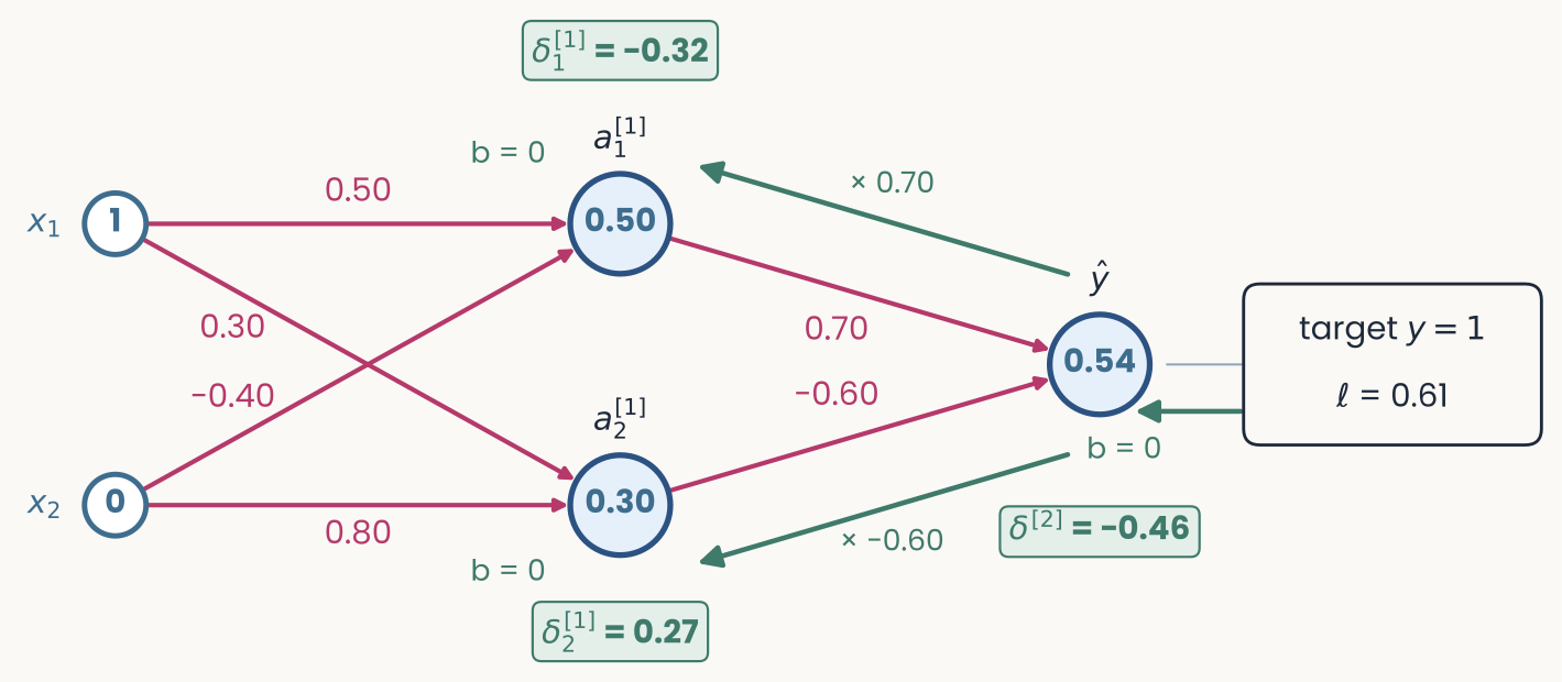
The same network. Green arrows run back from the output to each hidden unit, labelled times 0.70 and times minus 0.60. Green tags read delta 1 = minus 0.32 next to a1 of layer 1 and delta 2 = 0.27 next to a2 of layer 1
Open full-size figure

A hidden unit's error = output error × the linking weight × its ReLU slope $g'$ (1 if on, 0 if off)
$\textcolor{#3F7A6B}{\delta^{[1]}_1} = \textcolor{#3F7A6B}{\delta^{[2]}}\,\textcolor{#B5396B}{w^{[2]}_1}\,g'(z^{[1]}_1) = -0.46\times0.70\times1 = -0.32$ ; $\textcolor{#3F7A6B}{\delta^{[1]}_2} = -0.46\times(-0.60)\times1 \approx 0.27$
Each hidden unit gets its own error, even its own sign: $a^{[1]}_1$ should have been higher, $a^{[1]}_2$ lower

Return to contents

Slide 26

Step 4: every gradient is error × activity

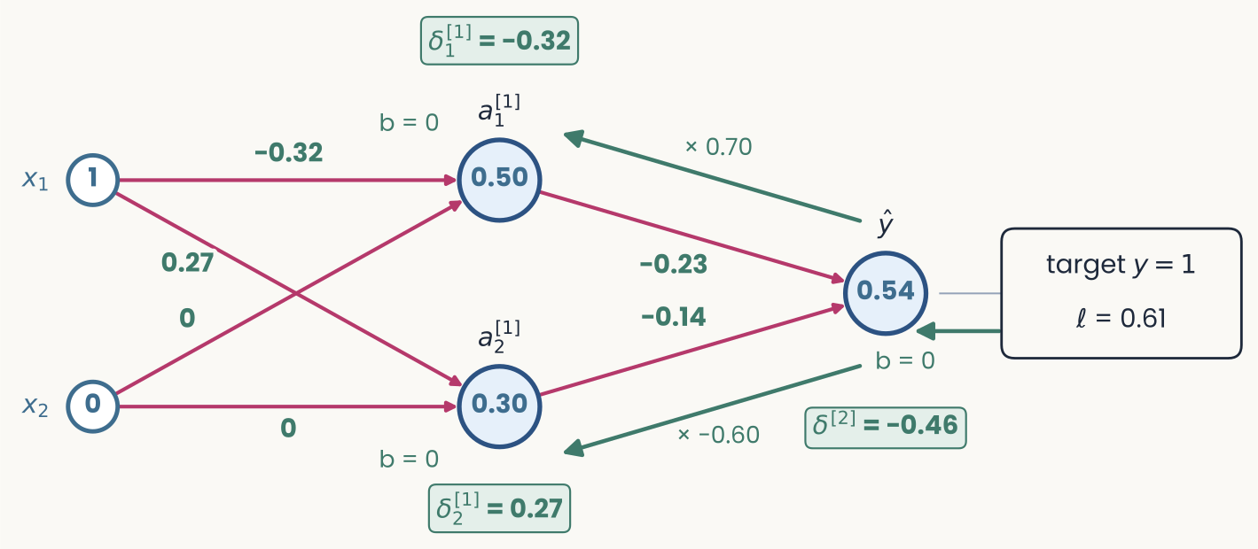
The same network with the weights replaced by their gradients in green: minus 0.32 and 0.27 on the connections from x1, 0 on both connections from x2, minus 0.23 and minus 0.14 on the connections into the output. The error tags stay in place
Open full-size figure

gradient = error × activity: $\partial\ell/\partial \textcolor{#B5396B}{w^{[2]}_1} = \textcolor{#3F7A6B}{-0.46}\times\textcolor{#3E6D8E}{0.50} = -0.23$
Weights from $x_2$ get 0, since $x_2 = 0$ . Each bias gets its unit's error: $-0.32$ , $0.27$ , $-0.46$
One step with $\eta = 1$ on all weights and biases: $\hat y$ rises from 0.54 to 0.82

Return to contents

Slide 27

Try it: train a small network on 2-D data

Compare one and two hidden units on XOR. Every weight is learned by the same four steps

Backpropagation playground: two classes of points in the plane (XOR, circles, two moons or spirals) and a small network with one or two hidden layers of ReLU units. Training runs backpropagation and gradient descent; the background colour shows the network's output, a gold line its decision boundary, and a curve the training loss as training goes on — open interactive version

Return to contents

Slide 28

Many classes: one output per class, then a softmax

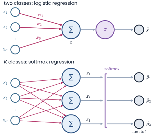
Two panels stacked. Top, two classes: inputs x1 to xD, each with its weight, summed into z, passed through a sigmoid to give one probability y-hat (logistic regression). Bottom, K classes: the same inputs feed three output neurons, each with its own weight vector w1, w2, w3, giving logits z1 to z3; a softmax turns them into three probabilities p-hat 1 to 3 that sum to 1 (softmax regression)

Open full-size figure

Top: one output, one probability. Bottom, $K$ classes: $K$ output units with their own weights, one weighted sum $z_c$ per class, the logits
Softmax: $\hat p_c = e^{z_c}/\sum_j e^{z_j}$ , which sum to 1
Loss $\ell = -\log \hat p_{\text{true}}$ ; error $\delta_c = \hat p_c - y_c$
Logits $(2,1,0)$ : $\hat{\mathbf p} = (0.67, 0.24, 0.09)$ ; $\ell = 0.41$ if class 1 is true
Right and confident, $\ell \to 0$ ; wrong and confident, $\ell$ grows without bound

Return to contents

Slide 29

The training loop

model   = nn.Linear(D, K)                  # D inputs, one logit for each of K classes
loss_fn = nn.CrossEntropyLoss()            # softmax + cross-entropy, averaged
opt     = torch.optim.SGD(model.parameters(), lr=0.1)   # SGD: a plain gradient step
for epoch in range(num_epochs):            # one epoch = one pass over the training set
    opt.zero_grad()                        # 1. clear the old gradients
    logits = model(X_train)                # 2. forward: logits for every image
    loss = loss_fn(logits, y_train)        # 3. the average cross-entropy
    loss.backward()                        # 4. gradient of the loss for every weight
    opt.step()                             # 5. update: w <- w - lr * gradient
with torch.no_grad():                      # evaluate on held-out images
    acc = (model(X_test).argmax(1) == y_test).float().mean()

One step: a batch of examples forward, their average loss, its gradient, an update. One epoch: every training example once. The model line alone sets a readout or a hidden layer
backward() computes the gradients. opt, the optimizer, turns them into weight changes in step()
Last lecture's learning cycle, now as code: forward, loss, gradient, step, repeat

Return to contents

Slide 30

Autograd: you never write the backward pass

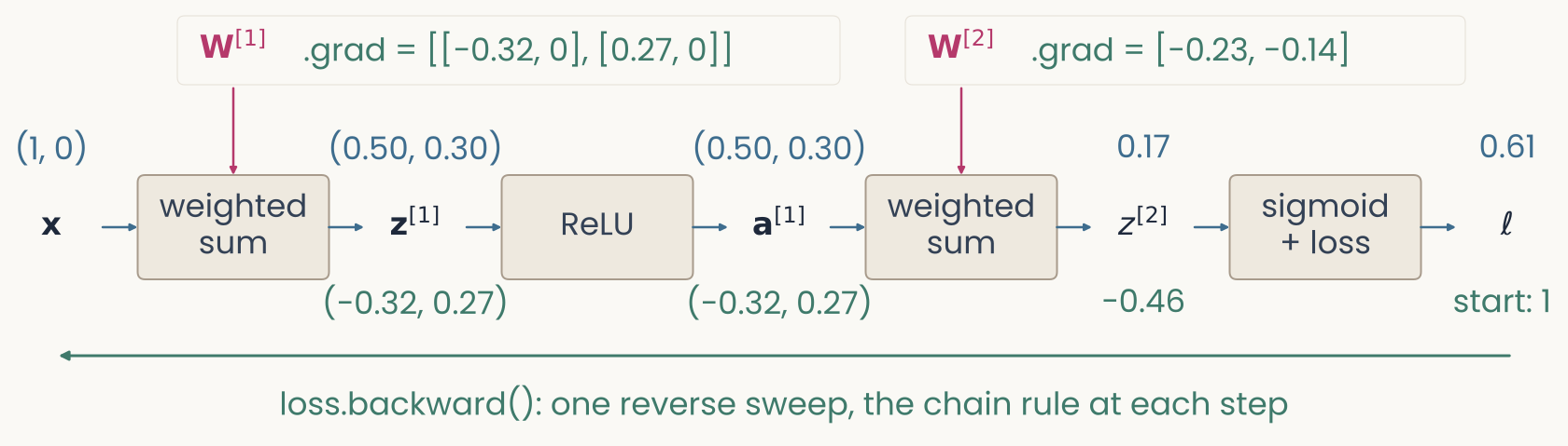
The worked example as PyTorch records it: x, a weighted sum with W1, z1, ReLU, a1, a weighted sum with W2, z2, and a sigmoid-plus-loss box giving ℓ. Forward values in blue above each quantity, gradients in green below, starting from 1 under ℓ; a long green arrow runs right to left, labelled loss.backward, one reverse sweep, the chain rule at each step. W1 and W2 carry their .grad values

Open full-size figure

PyTorch's automatic differentiation (autograd) records the forward pass as a computational graph: the operations that ran, and the values each one used
loss.backward() sweeps the graph in reverse: output error, hidden errors, then each parameter's gradient, stored in its .grad. opt.step() applies the update

Baydin, Pearlmutter, Radul & Siskind JMLR 2018

Return to contents

Slide 31

Reuse a trained network: transfer learning

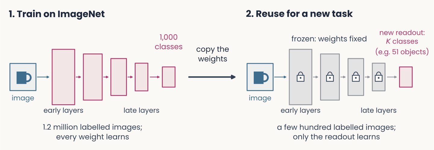
Two panels joined by an arrow labelled copy the weights. Left, 1, train on ImageNet: an image goes through a stack of layers, from early to late, to an output of 1,000 classes; 1.2 million labelled images, every weight learns. Right, 2, reuse for a new task: the same stack in grey with padlocks, frozen, weights fixed; the old output is replaced by a new readout for K classes, for example 51 objects; a few hundred labelled images, only the readout learns

Open full-size figure

Train once on a large dataset; freeze the layers and train only a new readout for the new task. A few hundred images can be enough

Return to contents

Slide 32

Train only part of a network

model = nn.Sequential(nn.Linear(D, 64), nn.ReLU(), nn.Linear(64, K))
model.load_state_dict(torch.load("trained.pt"))   # weights trained earlier
for p in model[0].parameters():            # the hidden layer
    p.requires_grad = False                # no gradients: these weights stay fixed
opt = torch.optim.Adam(model[2].parameters(), lr=1e-3)   # Adam: an optimizer, next lecture

model[0] is the first layer; .parameters() lists its weights and biases. The loop sets requires_grad = False on each: autograd computes no gradient for them, so they stay frozen
The optimizer is given only model[2], the readout: only its weights learn
Readout only: cheap. It shows what a trained readout can find in the hidden layer's fixed responses
Every weight: backpropagation also changes the hidden layer, so its responses to the images change too
Same data, same loss: only the set of weights allowed to move differs

Return to contents

Slide 33

Recap

One neuron: every learning rule moves the weights against the gradient of its loss, and the chain rule gives that gradient
Hidden layers: one neuron draws one line. Layers with a nonlinearity re-represent the inputs, so that a readout can separate classes no single line could
Backpropagation: forward pass, error at the output ( $\hat y - y$ ), error sent backward through the weights, and every gradient is error × activity. Autograd runs these steps for you
The training loop: forward, loss, backward(), step(), repeated over epochs, with a softmax output for many classes. Freezing trained layers reuses them for a new task

Return to contents

Slide 34

Minute paper

Submit on Canvas → Minute papers → Minute Paper 10 (access code read out in class).

Write three brief points in your own words:

In plain words, no equations: why can a multilayer perceptron solve XOR when a single neuron cannot?
Something you do not yet understand, or a question still open
Another idea you found interesting, and why it matters for brains, behavior or AI

Credit for a thoughtful attempt, not for being correct.

Return to contents

Slide 36

Going further

Optional slides, beyond the core of the lecture

Return to contents

Slide 37

Weight transport: must feedback copy the weights?

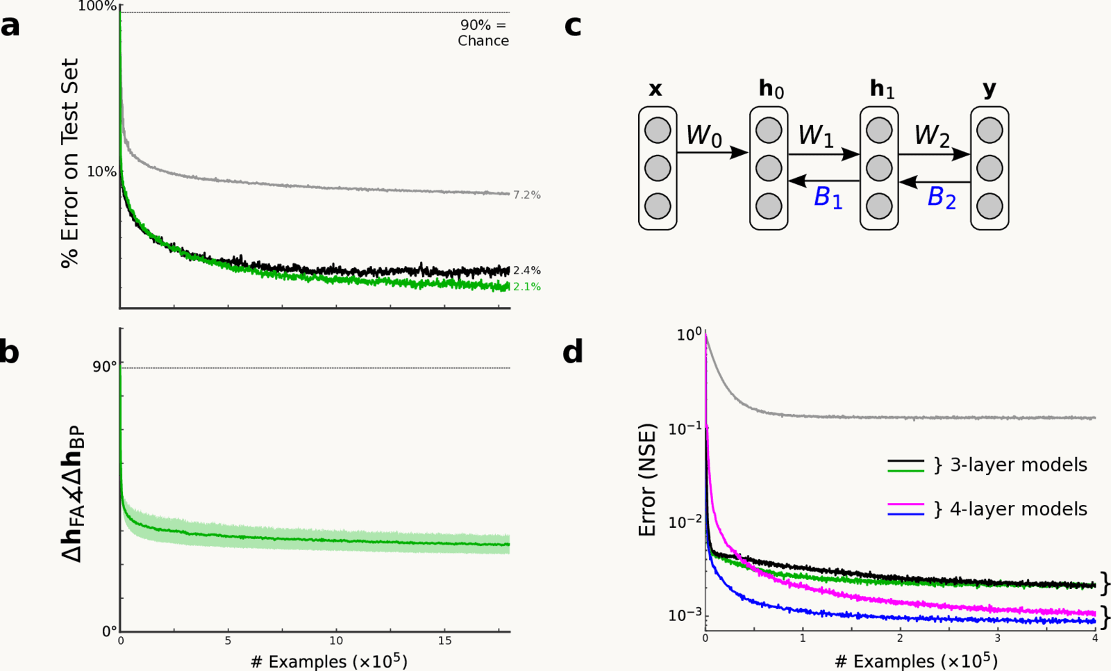
Feedback alignment, from Lillicrap et al. 2016, Fig. 2: with fixed random feedback weights the hidden-unit updates come within 90 degrees of backprop's, and the MNIST test error of feedback alignment nearly matches backprop's
Open full-size figure

Backprop sends the error back through the forward weights $\textcolor{#B5396B}{\mathbf{W}}^{\top}$ , so feedback synapses would have to copy them (weight transport)
With fixed random feedback weights $\mathbf{B}$ instead, the forward weights adapt until the hidden units' updates point within $90°$ of backprop's (panel b)
On MNIST (handwritten digits), 2.1% test error vs 2.4% for backprop

Lillicrap, Cownden, Tweed & Akerman Nat Commun 2016 · Whittington & Bogacz Neural Comput 2017 · Lillicrap et al. Nat Rev Neurosci 2020

Return to contents

Slide 38

Error signals in dendrites, one per neuron

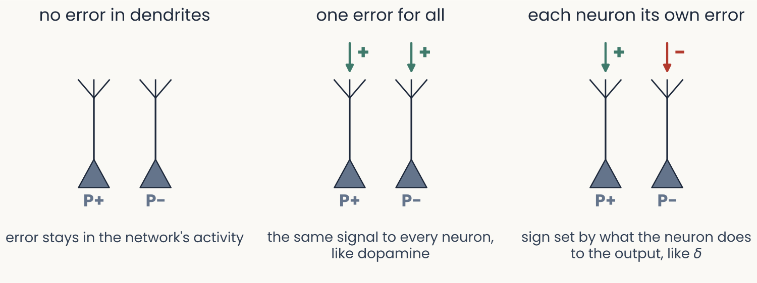
Three panels, each with two pyramidal neurons labelled P+ and P minus, with an apical dendrite rising to a tuft. No error in dendrites: no arrows. One error for all: the same green plus arrow onto both tufts, the same signal to every neuron, like dopamine. Each neuron its own error: a green plus arrow onto P+ and a red minus arrow onto P minus, sign set by what the neuron does to the output, like delta

Open full-size figure

Mice turned a grating with a brain–computer interface (BCI): a few layer-5 neurons (P+) rotated it toward the target, others (P−) away
Their apical dendrites carried error-related signals of opposite sign, matching each group's effect: each neuron its own error. Silencing them disrupted learning (caveat: a BCI task)

Francioni, Tang, Toloza, Ding, Brown & Harnett Nature 2026

Return to contents

Slide 39

Do backprop's gradients follow the brain's hierarchy?

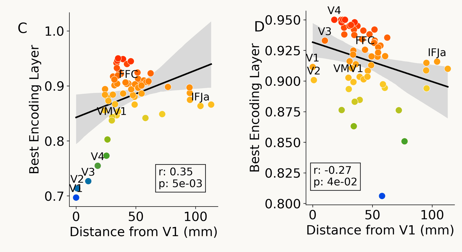
Two scatter plots, one point per brain region, horizontal axis distance from V1 in millimetres (0 to about 110), vertical axis the network layer that best predicts the region, as a fraction of network depth. Left, panel C, forward activations: V1, V2, V3 and V4 sit low near 0.7 to 0.77, regions farther from V1 are best predicted by deeper layers, and the fitted line rises (r = 0.35, p = 5e-03). Right, panel D, backpropagated gradients: V1 and V2 sit near 0.90 to 0.91, V4 near 0.95, and the fitted line falls with distance (r = -0.27, p = 4e-02)
Open full-size figure

Encoding models predicted fMRI from a network's activations and, separately, from its backpropagated gradients
Left, activations: regions farther from V1 match deeper layers. Right, gradients: the trend reverses
Shared representations, different ways of learning them?

Raugel et al. arXiv 2026

Return to contents

Hidden layers & backpropagation

Hidden layers & backpropagation

Last lecture: one neuron that learns

Learning the weights: start anywhere, walk downhill

You never see the whole landscape

The chain rule, one link at a time

The three links, worked out: delta rule

The three links, worked out: logistic regression

The perceptron is gradient descent after all

Why more than one layer?

One line fails on XOR; simpler rules do not

Stack them: two hidden units and one output

The hidden layer re-represents the input

Why the ReLU matters: linear layers collapse into one

With hidden layers, the landscape is no longer a bowl

How can a hidden unit learn when nothing tells it what to output?

Backpropagation: a long and disputed history

Notation for a network with layers

Nudge a hidden unit and follow the effect

Backpropagation: the recipe, for any network

Where the recipe comes from: the chain rule

Back to XOR: learn the weights from random ones

Step 1: the forward pass

Step 2: the error at the output

Step 3: send the error backward

Step 4: every gradient is error × activity

Try it: train a small network on 2-D data

Many classes: one output per class, then a softmax

The training loop

Autograd: you never write the backward pass

Reuse a trained network: transfer learning

Train only part of a network

Recap

Further reading for the research trail

Minute paper

Going further

Optional slides, beyond the core of the lecture

Weight transport: must feedback copy the weights?

Error signals in dendrites, one per neuron

Do backprop's gradients follow the brain's hierarchy?