The visual system & CNNs
Reader-friendly version of the 51 lecture slides: the lecture content in normal flow, with figure descriptions and data tables where the figure carries data. Open the presentation.
Slide 1

The visual system & CNNs
Slide 2
This week
- Exam 1: Thursday, in class. It covers the first eight lectures and the four steps of backpropagation
- Recitation tonight, 6:30 PM: exam preparation
- The third assignment is released Thursday
Slide 3
How do we make a network generalize better?
Regularization: any change to training that gives up some fit to the training data to do better on new data
Slide 8
Regularization 1: a penalty on the weights
Computed: the curve fit's 10 points, after Bishop (2006), Fig. 1.7
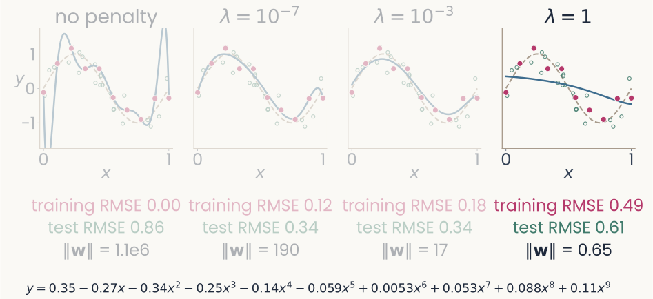
The same four panels, with the fourth panel, lambda equals 1, drawn in full and the others dimmed. Its fitted coefficients, written out below: y equals 0.35, minus 0.27 x, minus 0.34 x squared, minus 0.25 x cubed, minus 0.14 x to the fourth, minus 0.059 x to the fifth, plus 0.0053 x to the sixth, plus 0.053 x to the seventh, plus 0.088 x to the eighth, plus 0.11 x to the ninth. Under the panel: training RMSE 0.49, test RMSE 0.61, length of the weight vector 0.65. The point: every coefficient is under 0.35, the fitted curve is nearly a flat line, and the error rises on training and new points alike: too large a penalty underfits.
Open full-size figure- The fitted polynomial, λ = 1: every coefficient under 0.35, ‖w‖ = 0.65, and the curve is nearly flat
Slide 9
Ridge regression: the penalty on a neuron model
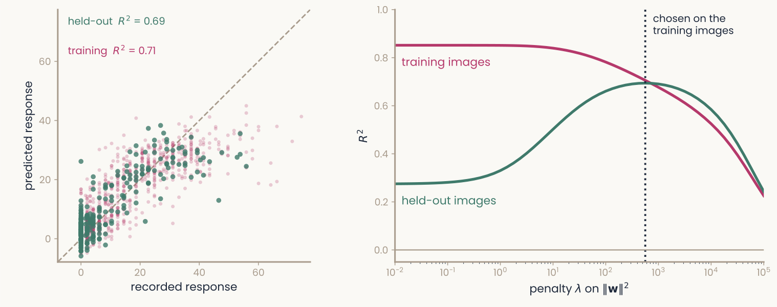
Computed: one monkey IT recording site (Bao et al., 2020) predicted from 512 units of an ImageNet-trained ResNet-18's late layer by ridge regression, a random fifth of the 1,224 images held out. Left panel: predicted response (vertical, 0 to 60) against recorded response (horizontal, 0 to about 75), with a dashed diagonal where the two are equal; faint magenta dots are training images, larger green dots held-out images, both spread along the diagonal. Labels: held-out R squared 0.69, training R squared 0.71. Right panel: R squared (vertical, 0 to 1) against the penalty lambda on a log axis from 10 to the minus 2 to 10 to the 5. With almost no penalty the magenta training curve is at 0.85 and the green held-out curve at 0.28; as the penalty grows they meet near 0.69 at a dotted vertical line, the lambda chosen by cross-validation within the training images, then both fall. The point: too small a penalty overfits, and the penalty is chosen without the held-out images.
Open full-size figureComputed: one monkey IT site (Bao et al. 2020), 1,224 object images, 512 late-layer units of ResNet-18; a random fifth held out
- Encoding model: one IT site from 512 units by ridge regression, λ by cross-validation inside the training images (
RidgeCV); too small a λ overfits (held-out 0.28 vs 0.69) - You fit this in the second assignment: one IT site, one layer. Assignment 3 scores such models of IT sites for two ResNet-50s, and the model–brain lecture runs it for every block
Slide 10
Regularization 2: dropout
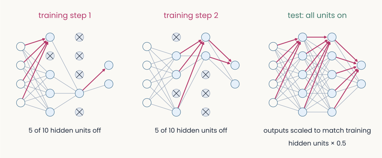
Schematic: three copies of the same small network, an input layer of four units, two hidden layers of five, and two output units, drawn as light blue circles joined by gray lines. Left, training step 1: five of the ten hidden units are crossed out and have no connections, one in the first hidden layer and four in the second. Middle, training step 2: a different five are crossed out, two in the first hidden layer and three in the second. Right, test: all units are on and every connection is drawn; caption, outputs scaled to match training, hidden units times 0.5. The point: at each training step a random half of the hidden units is switched off, so no unit can rely on a particular partner; at test time all are on.
Open full-size figure- Dropout: at each training step, switch off a random half of the hidden units; all are on at test time
- Often with the weight penalty, sometimes L1 (absolute values): each cuts the freedom to fit noise
Slide 15
Regularization 3: more examples
Computed: the same curve and noise, after Bishop (2006), Fig. 1.6
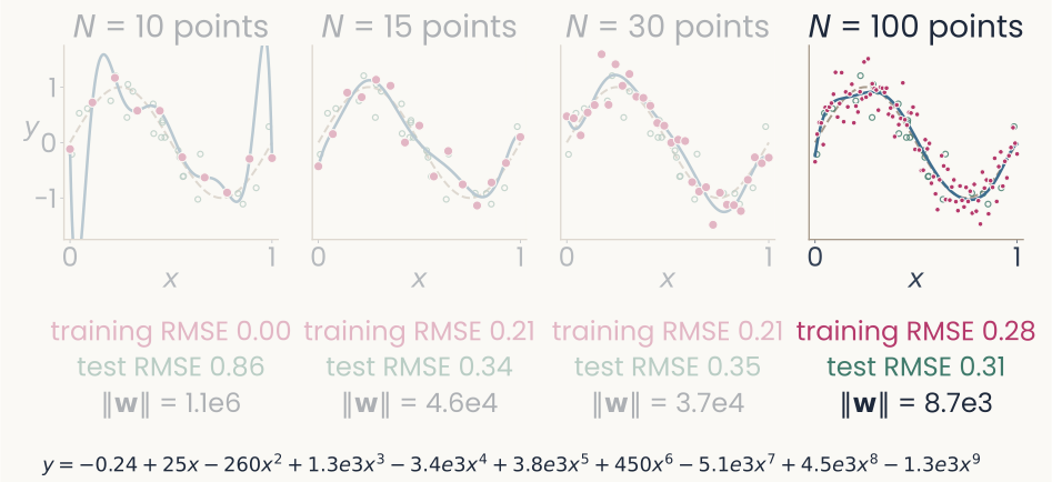
The same four panels, with the fourth panel, N equals 100 points, drawn in full and the others dimmed. Its fitted coefficients, written out below: y equals minus 0.24, plus 25 x, minus 260 x squared, plus 1.3 thousand x cubed, minus 3.4 thousand x to the fourth, plus 3.8 thousand x to the fifth, plus 450 x to the sixth, minus 5.1 thousand x to the seventh, plus 4.5 thousand x to the eighth, minus 1.3 thousand x to the ninth. Under the panel: training RMSE 0.28, test RMSE 0.31, length of the weight vector 8.7 thousand. The point: with 100 points the curve can no longer swing between them; the training error rises toward the noise level of 0.30 and the error on new points is the lowest of the four.
Open full-size figure- The fitted polynomial, N = 100: ‖w‖ = 8,700; with more points the curve stops swinging between them
Slide 16
No more data? Make altered copies of it
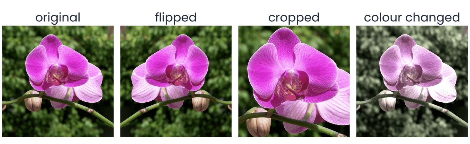
Computed with torchvision on one THINGSplus photograph of a pink orchid in front of dark green leaves. Eight square versions in two rows of four, each labeled above. Top row: Original; Horizontal flip, the mirror image; Resized crop, a zoomed-in part of the flower filling the square; Color jitter, the same view with shifted color and brightness. Bottom row: Rotation, the photo turned by a few tens of degrees with black corners; Affine warp, sheared and shifted with black wedges at the edges; Perspective, the photo squeezed as if seen at an angle inside a black frame; Random erasing, the original with a gray rectangle covering part of the flower. The point: every version still shows an orchid, so each can be a new training example with the same label.
Open full-size figure- Data augmentation: train on altered copies that keep the label: flips, crops, color, rotation, warps, erased patches. Choose transformations that should not change the label
Slide 17
Augmentation in PyTorch: a transform pipeline
transforms.Compose([
    transforms.RandomResizedCrop(224, scale=(0.5, 1.0)),  # Crop and resize
    transforms.RandomHorizontalFlip(),  # Flip horizontally at random
    transforms.RandomRotation(15),  # Rotate by up to 15 degrees
    transforms.ColorJitter(0.3, 0.3, 0.3, 0.05),  # Vary color and brightness
    transforms.ToTensor(),  # Convert to channel-first floats in [0, 1]
    transforms.Normalize(IMAGENET_MEAN, IMAGENET_STD),  # Standardize channels
])
- Each epoch draws a fresh random version of every image, so the network rarely sees the same picture twice. Flips that would change the label stay out: a 6 is not a 9
Slide 18
From the multilayer perceptron to the convolutional network
A dense layer on an image needs a weight for every pixel, and an object can appear anywhere: a small filter, applied at every position
Slide 19
Dense versus convolutional: where the weights go
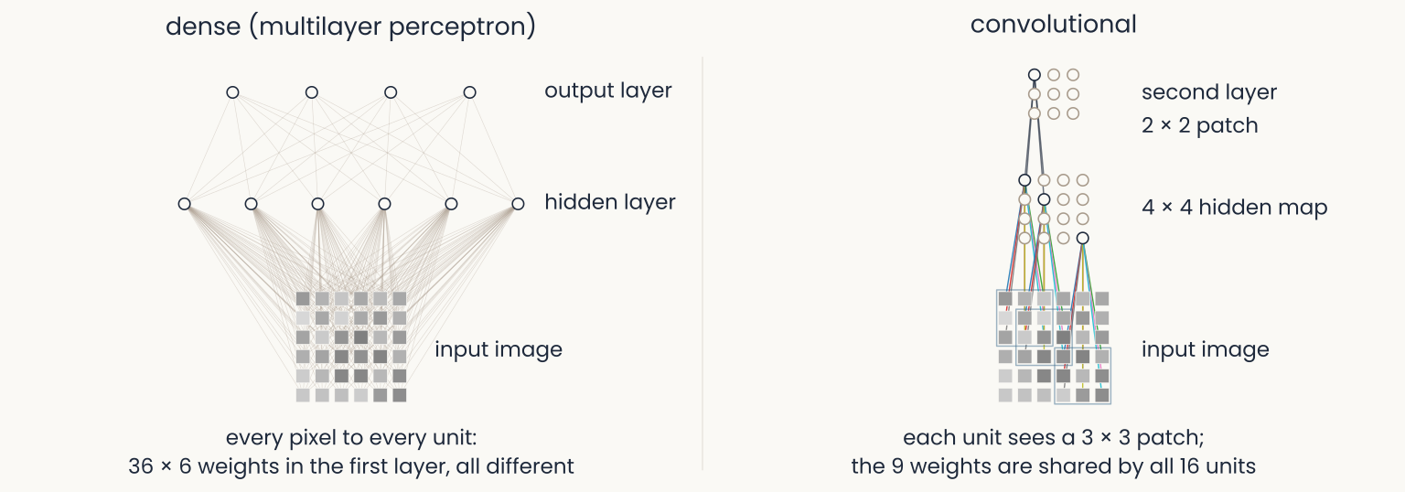
Schematic: two panels over the same 6 by 6 gray-level image, a grid of gray squares at the bottom of each. Left, dense (multilayer perceptron): six hidden units above the image, each joined to all 36 pixels by thin gray lines, a tangle of 216 lines, and four output units joined to all six hidden units; caption, every pixel to every unit, 36 times 6 weights in the first layer, all different. Right, convolutional: a 4 by 4 map of hidden units; three are drawn wired each to its own 3 by 3 patch of pixels, the nine lines in the same nine colors for every unit; above, a 3 by 3 second-layer map with one unit wired to a 2 by 2 patch of the first map; caption, each unit sees a 3 by 3 patch, the 9 weights are shared by all 16 units. The point: a convolutional layer wires each unit to a local patch and reuses the same weights at every position.
Open full-size figure- The perceptron wires every pixel to every unit. The convolutional layer wires each unit to a patch, and every unit shares the same weights: a feature detector copied across the image
Slide 20
Count the weights: a dense layer on an image
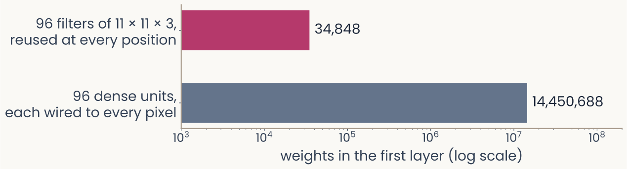
Computed: two horizontal bars on a log axis labeled weights in the first layer (log scale), from 10 to the 3 to 10 to the 8. Top bar, magenta: 96 filters of 11 by 11 by 3, reused at every position, 34,848 weights. Bottom bar, slate gray and much longer: 96 dense units, each wired to every pixel of a 224 by 224 color image, 14,450,688 weights. The point: on a log axis the dense layer's bar runs almost three decades further, about 400 times more weights for the same 96 units.
Open full-size figure- Flatten a 224 × 224 color image: one dense unit needs 224 · 224 · 3 = 150,528 weights, and it ignores which pixels are neighbors
- AlexNet's first layer instead learns 96 small filters of 11 × 11 × 3 and reuses each one at every position: 34,848 weights, about 400 times fewer than 96 dense units
- An object can sit anywhere in the image, so the detector is needed at every position: local filters, the same everywhere
Slide 21
Try it: template matching at every position
- The image is a grid of numbers; cut a 5 × 5 template, slide it: a dot product at each position. The best match is where it came from
Slide 22
Try it: slide the filter yourself
- One 7 × 7 filter, the tiger in 96 × 96 gray levels: step the window, read the dot product, watch the map fill in; then switch the filter
Slide 23
Convolution: one filter, slid over the image
- A filter (or kernel), a small grid of weights, a template, slid over the image; at each position the dot product, then ReLU: a feature map. Shift the image and the map shifts with it
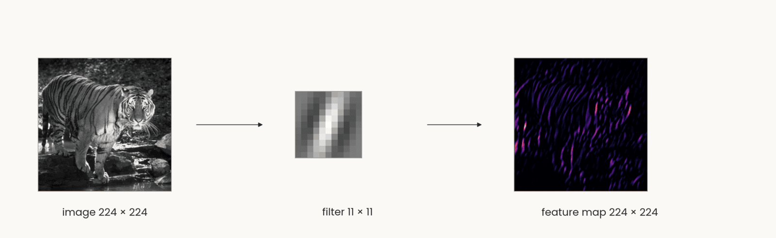
Computed. Three items left to right joined by arrows. The tiger photograph in gray levels, labeled image 224 by 224. An 11 by 11 Gabor filter, labeled filter 11 by 11: a small grid of gray squares with a bright stripe between two dark stripes, tilted about 20 degrees from vertical. The feature map, labeled feature map 224 by 224: a dark square with bright magenta and orange streaks wherever the tiger has stripes at the filter's orientation, mostly on the body and legs. The point: one set of weights is applied at every position, and the map keeps the image's layout, so shifting the image shifts the map.
Open full-size figureSlide 24
One filter gives one map; a layer gives a stack of maps
- Four filters, four feature maps: the layer's output is a stack, one channel per filter, 224 × 224 × 4. Channels are the depth of the next layer's input
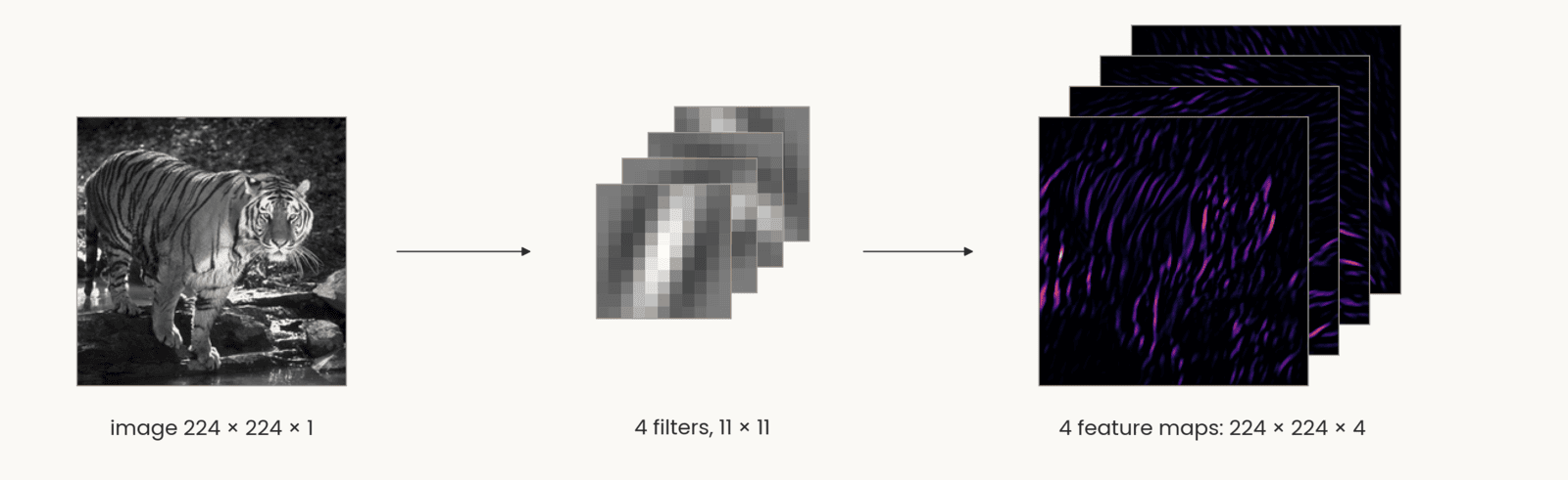
Computed: the same tiger photograph, labeled image 224 by 224 by 1, an arrow to four 11 by 11 Gabor filters at four orientations stacked as offset cards, labeled 4 filters, 11 by 11, and an arrow to four feature maps stacked as offset cards in the same dark-to-orange color map as the single map before, labeled 4 feature maps: 224 by 224 by 4. The front map shows the near-vertical stripes; the maps behind it respond to the other three orientations. The point: each filter gives one map, so the layer's output is a stack with one channel per filter, and that stack is the next layer's input.
Open full-size figureComputed: the tiger, four 11 × 11 Gabor filters, stride 1, padding 5, ReLU
Slide 25
The convolutional layer, in notation
Schematic: two panels over the same 6 by 6 gray-level image, a grid of gray squares at the bottom of each. Left, dense (multilayer perceptron): six hidden units above the image, each joined to all 36 pixels by thin gray lines, a tangle of 216 lines, and four output units joined to all six hidden units; caption, every pixel to every unit, 36 times 6 weights in the first layer, all different. Right, convolutional: a 4 by 4 map of hidden units; three are drawn wired each to its own 3 by 3 patch of pixels, the nine lines in the same nine colors for every unit; above, a 3 by 3 second-layer map with one unit wired to a 2 by 2 patch of the first map; caption, each unit sees a 3 by 3 patch, the 9 weights are shared by all 16 units. The point: a convolutional layer wires each unit to a local patch and reuses the same weights at every position.
Open full-size figure- Left, the MLP layer: every input to every unit. Right, the convolution: each unit sees a patch of all input maps, the same weights at every position
- : the filters, of them, each ; : the feature maps, one channel per filter
Slide 26
Which brain areas turn an image into an object?
Simple and complex cells: the weighted sum and the pooling of the last slides, found in cortex decades earlier
Slide 27
Core object recognition: animal or not?
Slide 28
Monkeys do it too
- Monkeys trained on the task answer as fast as people. From a few electrodes over V4 and posterior IT, a linear readout recovers the category, and it errs on the same images as the monkeys
Slide 29
The ventral stream: a hierarchy of areas
- Tuning gets more complex (edges, parts, objects) and more tolerant of position and size
- In IT, a linear readout of ~100 neurons reports the category: a linear classifier separates the categories
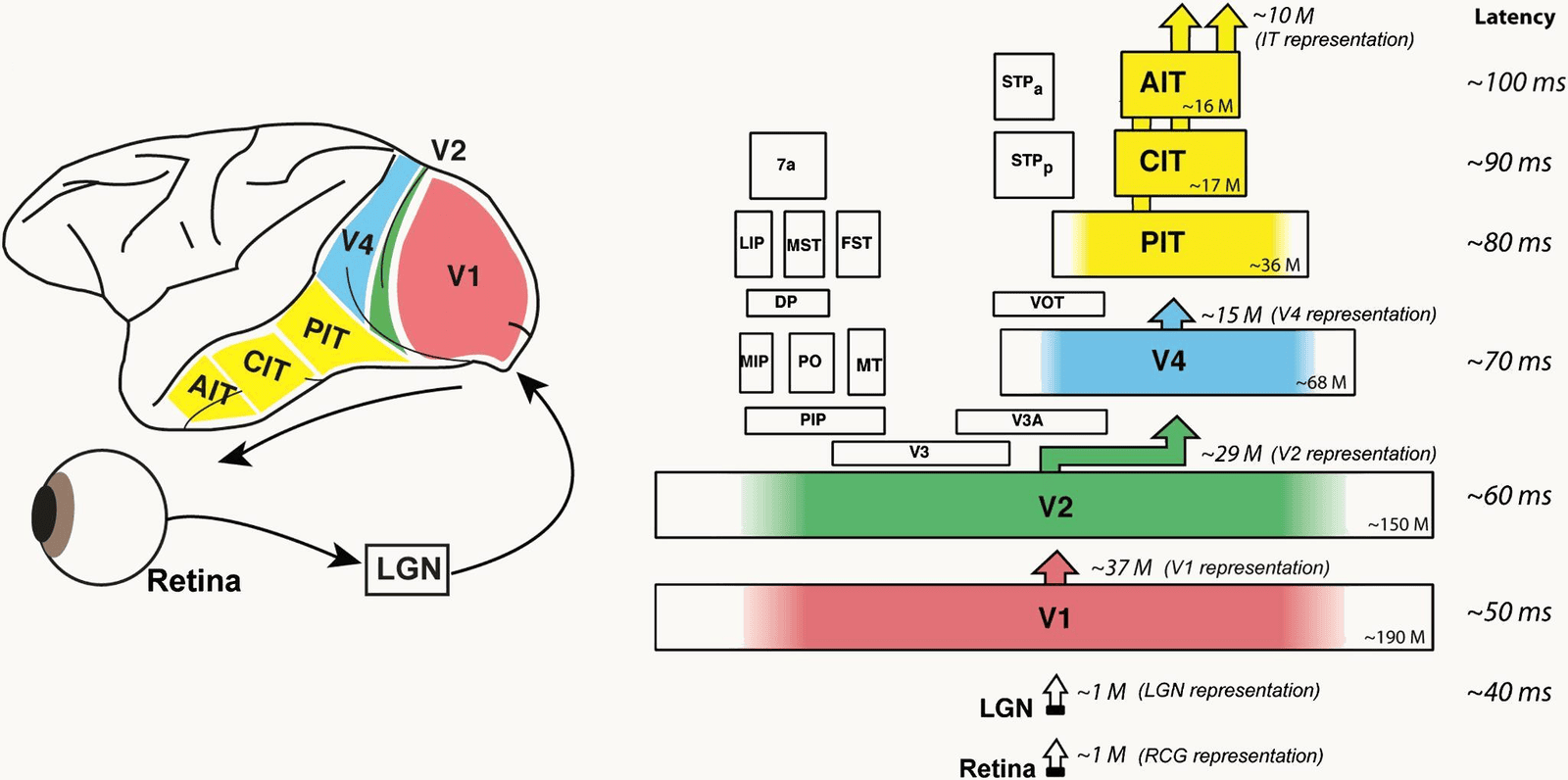
DiCarlo, Zoccolan and Rust (2012), Figure 1. Left: a side view of the macaque brain with the ventral visual stream colored, V1 in red at the back, V2 green, V4 blue, and the inferior temporal cortex in yellow divided into PIT, CIT and AIT toward the front; below, an eye, an arrow to a box labeled LGN, and an arrow from the LGN to V1. Right: the same areas stacked as boxes from bottom to top with the typical response latency beside each: LGN about 40 milliseconds, V1 about 50, V2 about 60, V4 about 70, PIT about 80, CIT about 90, AIT about 100. Each box carries an approximate neuron count, from about 190 million in V1 to about 16 million in AIT, and arrows between stages give the size of each representation, from about 1 million at the LGN to about 10 million at IT. The point: the ventral stream is a hierarchy of areas, each adding about 10 milliseconds.
Open full-size figureSlide 30
Retina and LGN: Kuffler's center–surround cells
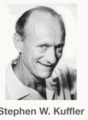
A black-and-white head-and-shoulders photograph of Stephen W. Kuffler, the physiologist who mapped the center-surround receptive fields of retinal ganglion cells in 1953. An older man with a high forehead and receding hair, smiling broadly, in a light open-collared shirt, looking slightly to the left of the camera. His name is printed under the photograph. The portrait sits in the top-right corner of the slide, above the caption Stephen Kuffler.
Open full-size figure- A cell's receptive field: the patch of the visual field where light changes its firing. For a retinal ganglion or LGN cell, light on the + center excites, on the − surround inhibits (left: on-center, and its mirror image, off-center); uniform light does nothing. Right, Kuffler's records: these cells report local contrast, not brightness
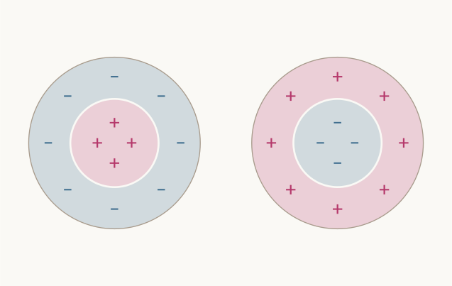
Schematic: two circular receptive fields side by side. Left, an on-center cell: a pink inner disc marked with three magenta plus signs, inside a light blue ring marked with four blue minus signs. Right, an off-center cell, the reverse: a light blue inner disc with minus signs inside a pink ring with plus signs. No labels. The point: light on the plus region raises the cell's firing and light on the minus region lowers it, so uniform light over both does almost nothing.
Open full-size figure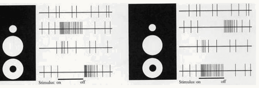
Kuffler's 1953 recordings as redrawn in Hubel's book Eye, Brain and Vision. Two panels, each a black rectangle with three white stimuli, a small spot, a larger spot and a ring, beside four rows of spike records; a bar under the records marks when the stimulus is on and off. Left panel, an on-center retinal ganglion cell: the top row is the resting discharge with no stimulus; the small spot on the center gives a dense burst while the light is on; the larger spot covering center and surround gives only a few spikes; the ring on the surround silences the cell while on and gives a burst at off. Right panel, an off-center cell, the mirror image: the small spot silences the cell and gives a burst at off, the large spot does little, the ring gives a burst while on. The point: these cells report local contrast, not brightness.
Open full-size figureSlide 31
V1: Hubel & Wiesel's recording, on film
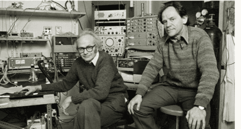
A black-and-white photograph of David Hubel and Torsten Wiesel in their laboratory, surrounded by racks of recording equipment, oscilloscopes and amplifiers. Hubel, wearing glasses and a dark sweater, sits on the left with one hand on the apparatus; Wiesel, in a patterned sweater, sits on a stool on the right. Both look toward the camera. The portrait sits in the top-right corner of the slide, above the caption Hubel and Wiesel.
Open full-size figure- One neuron in cat V1, one electrode, a bar of light moved by hand: the clicks are its spikes, and they come only for the right orientation at the right place
Slide 32
V1: Hubel & Wiesel's oriented cells
A black-and-white photograph of David Hubel and Torsten Wiesel in their laboratory, surrounded by racks of recording equipment, oscilloscopes and amplifiers. Hubel, wearing glasses and a dark sweater, sits on the left with one hand on the apparatus; Wiesel, in a patterned sweater, sits on a stool on the right. Both look toward the camera. The portrait sits in the top-right corner of the slide, above the caption Hubel and Wiesel.
Open full-size figure- Hubel & Wiesel mapped V1 cells by hand (left; crosses excite, triangles inhibit). Right, the same maps a–g as + and − regions: center–surround (a, b), bar detectors (c, d, e, f) and an edge detector (g), each at one orientation
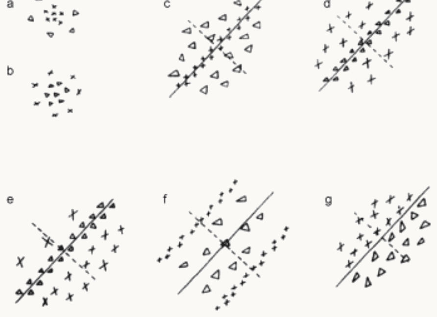
Hubel and Wiesel (1962), Text-figure 2: seven receptive fields of cat cells mapped by hand with spots of light, labeled a to g. In the source's legend, crosses mark areas giving excitatory (on) responses and triangles areas giving inhibitory (off) responses; a continuous line through each elongated field marks its axis. Panels a and b, stacked at the left, are circular: a has crosses in the center inside a ring of triangles, on-center; b the reverse, off-center. Panels c to g are elongated along an oblique axis: c has a narrow stripe of crosses between flanks of triangles; d, e and f have a stripe of triangles between flanks of crosses; g has crosses on one side of the axis and triangles on the other, an edge. The point: cortical receptive fields are parallel excitatory and inhibitory strips at one orientation, not concentric rings.
Open full-size figure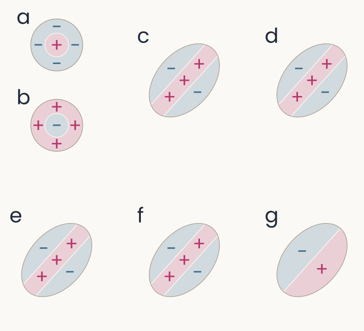
Schematic redrawing of the seven hand maps a to g with pink plus regions and light blue minus regions. Panels a and b at the left are circles: a, a pink plus center inside a blue minus ring, on-center; b, a blue minus center inside a pink plus ring, off-center. Panels c, d, e and f are ellipses tilted about 48 degrees, each with a pink plus stripe along the long axis between two blue minus flanks. Panel g is an ellipse split along its long axis, blue minus on the upper-left half and pink plus on the lower-right half, an edge. The point: each oriented cell sums light with positive weights along a stripe and negative weights beside it.
Open full-size figureSlide 33
V1 in one picture: ganglion → simple → complex
- Left to right, ganglion or LGN cells, simple cells, complex cells: center–surround → oriented at one position → oriented anywhere nearby: a weighted sum, then a pooling, the two operations every stage of today's models repeats
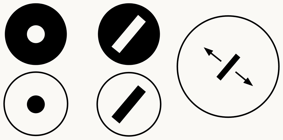
Three columns of black-and-white icons summarizing Hubel and Wiesel's V1. Left column, retinal ganglion or LGN cells: a black disc with a white spot in the center, an on-center cell, above a white disc with a black spot, an off-center cell. Middle column, simple cells: a black disc with a white oblique bar, above a white disc with a black oblique bar, each oriented and at one position. Right column, a complex cell: one large circle with a black oblique bar in the middle and a double-headed arrow across it, showing the bar can sit anywhere in the field at that orientation. The point: a weighted sum builds selectivity for orientation, and a pooling builds tolerance to position.
Open full-size figureSlide 40
Mechanism: a row of LGN cells makes a simple cell
- Shifted further: the bar must line up with the + centers
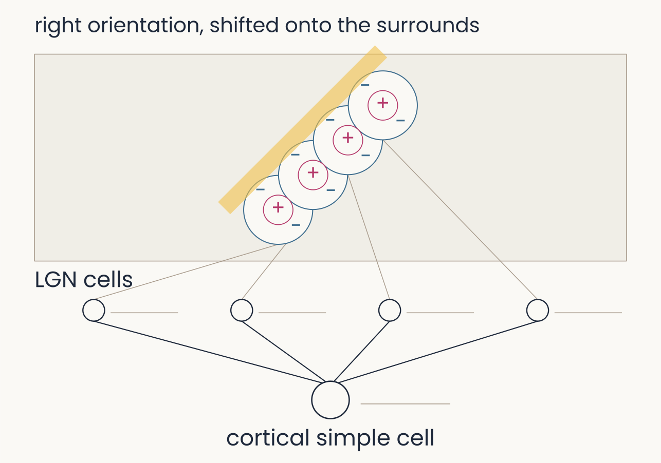
The same four model LGN cells converging on a cortical simple cell, with the bar at the row's orientation but shifted sideways by 0.8 units, now almost clear of the fields along their upper-left edge; the frame is labeled right orientation, shifted onto the surrounds. Spike trains: all four LGN cells and the simple cell show no spikes. The point: a simple cell is selective for position as well as orientation, because the bar must line up with the plus centers.
Open full-size figureSlide 47
Mechanism: simple cells converge on a complex cell
- Past the fields: each simple cell covers a narrow range, the complex cell a broad one
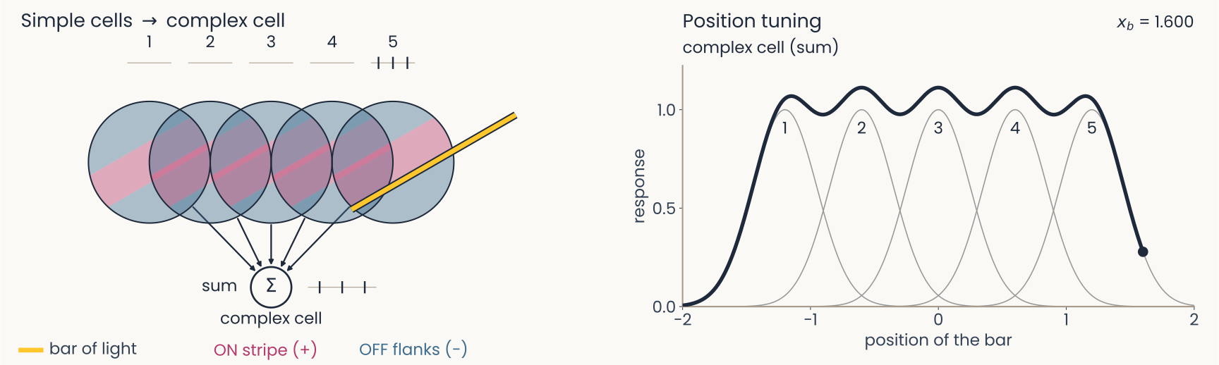
The same five model simple cells converging on a complex cell, with the bar past the right edge of field 5 at position 1.600. Spike trains: cell 5 three spikes, the others none, the complex cell three. Right panel: the dark complex-cell curve is now drawn over the whole range from minus 2 to 2: it rises from zero near minus 1.6, stays between about 0.98 and 1.1 across the five preferred positions with small dips between them, and falls back to zero past 1.6, while each gray simple-cell curve covers only a narrow range of positions. The point: each simple cell covers a narrow range of positions and the complex cell, their sum, a broad one, at the same orientation.
Open full-size figureSlide 48
Recap
- Generalize better: a penalty on the weights (weight decay, ridge), dropout, more or altered data, with λ chosen on validation data
- Brain: center–surround, simple cells wired from rows of LGN cells, complex cells that pool them; receptive fields mapped by hand or by reverse correlation
- Network: convolution (one filter, shared across positions) is the simple cell's weighted sum; pooling over nearby positions is the complex cell
Slide 49
Further reading for the research trail
Optional: a few research-trail entries over the semester. Any paper mentioned in any lecture qualifies.
- Fukushima Biol Cybern 1980: the Neocognitron, the first S/C hierarchy, trained without labels
- Serre & Poggio Commun ACM 2010: HMAX and the table of data it accounts for, from V1 to behavior
- Linsley, Feng & Serre Trends Cogn Sci 2026: why better AI stopped meaning better models of biology
- Cammarata et al. Distill 2020: curve detectors, one family of units in InceptionV1 followed from feature visualization to circuit
- Yamins et al. PNAS 2014: networks that recognize objects better also predict IT neurons better
Slide 50
Further reading, continued
- Zhuang et al. PNAS 2021: networks trained without labels predict ventral-stream neurons as well as labeled ones
- Konkle & Alvarez Nat Commun 2022: a network trained without labels matches human ventral fMRI
- Kar et al. Nat Neurosci 2019: images that IT solves late, which feedforward networks miss
- Jinsi, Henderson & Tarr PLOS ONE 2023: starting on blurred images helps a network learn categories
- Lu et al. Nat Mach Intell 2026: an infant-like visual diet gives shape-based, robust networks
Slide 51
Minute paper
Submit on Canvas → Minute papers → Minute Paper 12 (access code read out in class).
Write three brief points in your own words:
- Hubel and Wiesel's simple and complex cells each correspond to one operation of a convolutional
network. Name the two operations, and say what each buys the network. - Something you do not yet understand, or a question still open
- Another idea you found interesting, and why it matters for brains, behavior or AI
Credit for a thoughtful attempt, not for being correct.