Large language models and the brain
Reader-friendly version of the 55 lecture slides: the lecture content in normal flow, with figure descriptions and data tables where the figure carries data. Open the presentation.
Slide 1

Large language models and the brain
Slide 3
Finish the sentence
He spread the warm bread with ___
- Most of you thought butter: you predicted the next word, as our language models do
- socks (from the attention lecture) → larger EEG response ~400 ms after the word: the N400
- A language model assigns every word a surprisal (how unexpected it is). Does surprisal predict reading times and N400 size?
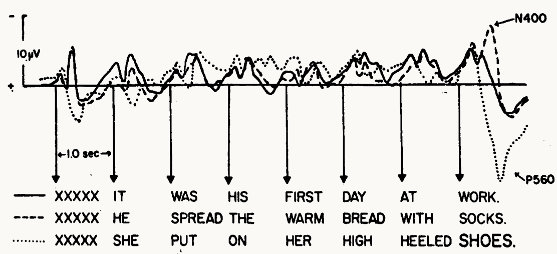
Published figure: Figure 1A of Kutas and Hillyard (1980), Science. Average EEG recorded at the back of the scalp while people read three seven-word sentences, one word per second. The horizontal axis is time, with the onset of each word marked by an arrow and the words printed below; a bracket marks 1.0 second. The vertical axis is voltage, with a 10 microvolt scale bar and negative plotted upward. Three traces are drawn, one per sentence: a solid line for It was his first day at work, a dashed line for He spread the warm bread with socks, and a dotted line for She put on her high heeled SHOES, whose last word is printed in large type. The three traces are similar through the first six words. After the last word, the solid trace stays near baseline. The dashed trace swings to a large negative peak about 400 ms after socks, labeled N400. The dotted trace swings the other way, to a positive peak labeled P560. The slide uses this to show that a word that does not fit its sentence produces a larger N400, the response that surprisal is later compared with.
Open full-size figureSlide 4
Scaling up the language model
The same transformer, trained on more text than anyone could read
Slide 5
Where we left off
- Next-token transformers are generative models: sample a token, append it, repeat → text. Same principle behind image and video generators, and world models (later in the course)
- Transformer + self-supervised training (as in vision) → here the target is the next token, so any text is training data (pretraining)
- Today: (1) scaling up: scaling laws, tokens, data, in-context learning, assistants (instruction tuning, RLHF, tools); (2) large language models (LLMs) as models of readers and brains: surprisal, reading times, the N400, encoding models; (3) predictive coding
Slide 6
Scaling laws: the loss falls smoothly with size
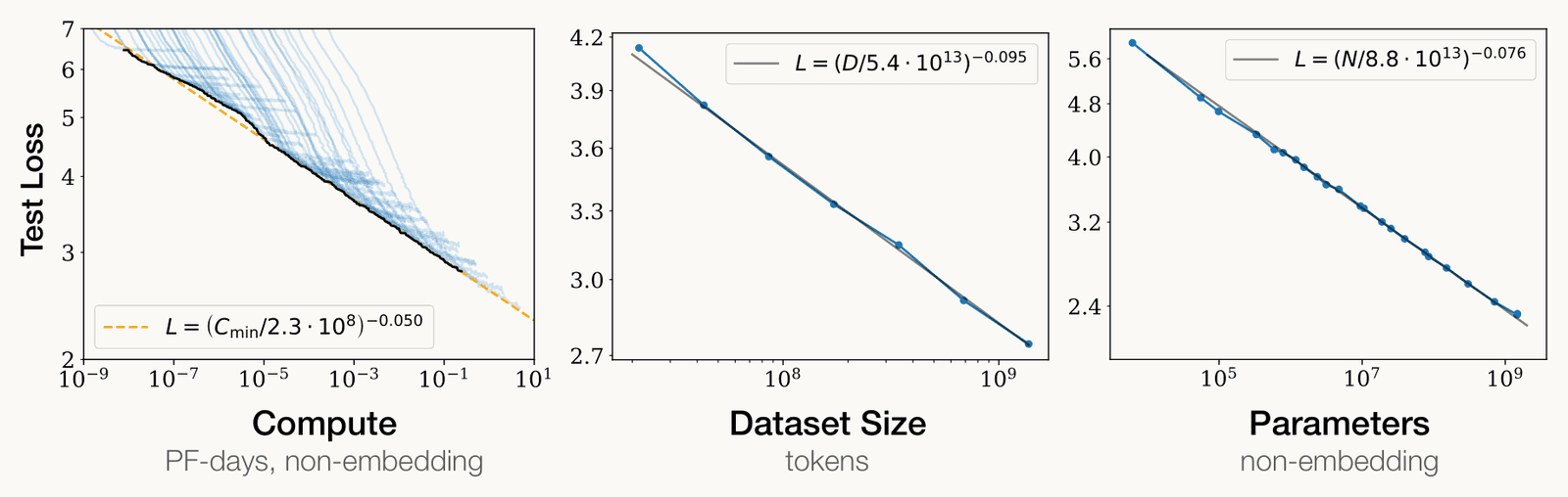
Published figure: Figure 1 of Kaplan et al. (2020), Scaling laws for neural language models. Three side-by-side line plots, each with both axes on a logarithmic scale and the language model's test loss (cross-entropy, from about 2 to 7) on the vertical axis. Left panel: loss against compute in petaflop-days, from 10 to the minus 9 up to 10, drawn as many pale blue training curves with a black lower envelope and an orange dashed power-law fit, loss = (compute / 2.3 times 10 to the 8) to the power minus 0.050. Middle panel: loss against dataset size in tokens, from about 2 times 10 to the 7 to 2 times 10 to the 9, with six blue points falling from about 4.1 to 2.7 along a grey line with exponent minus 0.095. Right panel: loss against non-embedding parameters, from about 10 to the 3 to 10 to the 9, with many points falling from about 5.6 to 2.3 along a grey line with exponent minus 0.076. On a log-log plot a power law is a straight line, and all three are straight over several orders of magnitude. The slide uses this to show that loss falls smoothly and predictably as compute, data or parameters grow.
Open full-size figure- A striking finding of modern AI: test loss (cross-entropy, held-out text) falls predictably with scale, a power law (line on log–log axes) in compute (PF-days), data, parameters. Left: one curve per model size; black = best loss
- Why a law? A frontier run takes months → fit small runs first and predict the large run's loss before committing
Slide 7
From characters to word pieces
- Scale is counted in tokens and parameters. Token = the unit the transformer reads: characters in our assignment model, word pieces in GPT-2. How is the vocabulary chosen?
- Byte-pair encoding (BPE):
- Start with all 256 possible byte values (letters, digits, punctuation, and pieces of other characters)
- Count every pair of neighboring tokens in a large text; merge the most frequent pair into one new token (
t+h→th) - Repeat: merged tokens can merge again (
th+e→the); old tokens stay - Stop at the chosen vocabulary size
Slide 8
Word pieces in GPT-2
- Frequent words → one token; rare strings stay in pieces:
brain,neuroscience→ one token each ·tokenization→token+ization·surprisal→surpr+isal· the made-upZorblat→Z+or+bl+at - GPT-2: 256 bytes + 50,000 merges + 1 end-of-text token = 50,257 tokens
- Vocabulary sizes range ~8×, in tokens: Llama 2 32 K · GPT-2 50 K · GPT-4 ~100 K · Llama 3 128 K · Qwen2.5 ~152 K · GPT-4o ~200 K · Gemma 256 K
- Larger vocabulary → fewer tokens per text, better coverage of other languages
- Rule of thumb for English: 1 token ≈ 0.75 words (100 tokens ≈ 75 words)
Slide 9
How much text do modern LLMs use?
Data, the first ingredient of scale, counted in tokens: how much do models read?
- Llama 3 (Meta, 2024): ~15 T tokens ≈ 130 M books, about every book ever published
- Newer open models:
- Qwen3 (Alibaba, 2025): ~36 T tokens
- Llama 4 (Meta, 2025): > 30 T tokens of text, images and video
- DeepSeek-V3 (2024): 14.8 T tokens; later V3 versions continue from it
- The web: ~510 T tokens indexed by search engines, ~3,100 T in all; ~300 T of usable public text → used up between 2026 and 2032 at the current pace
- A child hears ~130 M tokens by age 13 → Llama 3 reads ~100,000× more
T = trillion · B = billion · M = million · web figures are estimates
Slide 10
Model size: the largest are undisclosed
| Model | Year | Built by | Training tokens | Parameters |
|---|---|---|---|---|
| GPT-2 | 2019 | OpenAI | ~0.01 T | 0.1 – 1.5 B |
| GPT-3 | 2020 | OpenAI | 0.3 T | 175 B |
| Chinchilla | 2022 | DeepMind (Google) | 1.4 T | 70 B |
| Llama 3 | 2024 | Meta | 15 T | 8 – 405 B |
| Frontier models | 2023 on | OpenAI, Google, … | ? | ? |
- Frontier models: the most capable ones (GPT, Claude, Gemini), closed, size and data undisclosed
- A growing gap: academic labs, including brain research, use open models (GPT-2, Pythia, Llama, OLMo), far below the frontier in scale and ability
Slide 11
Compute: the third ingredient
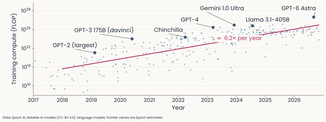
Figure computed for this lecture from Epoch AI's Notable AI Models dataset (CC-BY 4.0, downloaded 2026-11-17), language models only. A scatter plot. The horizontal axis is publication year, 2017 to 2026. The vertical axis is training compute in floating-point operations (FLOP), on a logarithmic scale with gridlines at 10 to the 16, 19, 22, 25 and 28. Each small blue dot is one model, 286 in all. A magenta line is the least-squares fit of log compute against date for the 276 models from 2018 on; it rises about 6.2 times per year, a doubling every 4.6 months. Seven models are labeled with larger dots: GPT-2 (largest) in 2019 at about 2 times 10 to the 21, GPT-3 175B in 2020 at about 3 times 10 to the 23, Chinchilla in 2022 at about 6 times 10 to the 23, GPT-4 in 2023 at about 2 times 10 to the 25, Gemini 1.0 Ultra in late 2023 at about 5 times 10 to the 25, Llama 3.1-405B in 2024 at about 4 times 10 to the 25, and GPT-6 Astra in 2026 at about 9 times 10 to the 26, the highest point. The compute of the frontier models is Epoch's estimate, since the labs do not publish it. From GPT-2 to GPT-6 Astra, training compute grows about 500,000 times. The slide uses this to show compute as the third ingredient, after data and parameters, in the growth of language models.
Open full-size figure- Training compute of language models: ~6× more every year (fit to 276 models, 2018–2026) → GPT-2 to today's largest: ~500,000× in seven years
Slide 12
Scaling laws in practice
Data, parameters, compute: how should a fixed compute budget be split between model size and data?
- Chinchilla (2022): a fixed compute budget buys a bigger model or more training text (cost ∝ parameters × tokens)
- Gopher: big model, 280 B parameters, trained on 300 B tokens
- Chinchilla, same cost: 4× smaller (70 B), so it can read ~5× more new text (1.4 T tokens) → lower loss
- Gopher was too big for its data. Rule: ~20 training tokens per parameter (1.4 T ÷ 70 B)
- Yet small models are trained far past this (Llama 3 8B: 15 T tokens ≈ 1,900 per parameter): a bigger model would be better for the same training cost, but a small one is cheaper to run each time it answers, over billions of questions
- Lower loss ≠ ability, yet abilities thought to need special architectures came with scale → the bitter lesson: general methods that use more compute win (Sutton 2019)
Slide 13
Do large models converge?
As models scale, do they also become alike?
- Take images with their captions. A vision model (images only) and a language model (captions only) each group similar items: dog near wolf, far from car. The bigger the two models, the more their groupings agree
- Platonic representation hypothesis: scale drives models toward one shared statistical model of reality, the process that generated the data
- Debated: the evidence rests on a few alignment measures, and counterexamples exist
- If true → a brain, shaped by the same world, might converge on the same representation. Later today: language models compared with brains
Slide 14
In-context learning: what a prompt looks like
- Before GPT-3: new task → fine-tuning: keep training the pretrained weights on labeled examples of that task (like readouts on vision networks). A pretrained model reused this way is a foundation model
- In-context learning: give the task in the prompt, weights fixed → one model, many tasks (as people learn a task from a few examples)
- Example task, never trained for: remove the random symbols from a word
-
Zero-shot: the instruction, no examples → relies on pretraining (instructions followed by answers are common in web text)
Remove the symbols from the word. b!r.a/i n = -
Few-shot: a few solved examples, then a new word (one example: one‑shot)
s.u!c/c!e.s s i/o/n = succession·p,l.a!n e/t = planet·b!r.a/i n = -
The model continues the text with
brain: only the examples tell it the rule
-
Slide 15
In-context learning
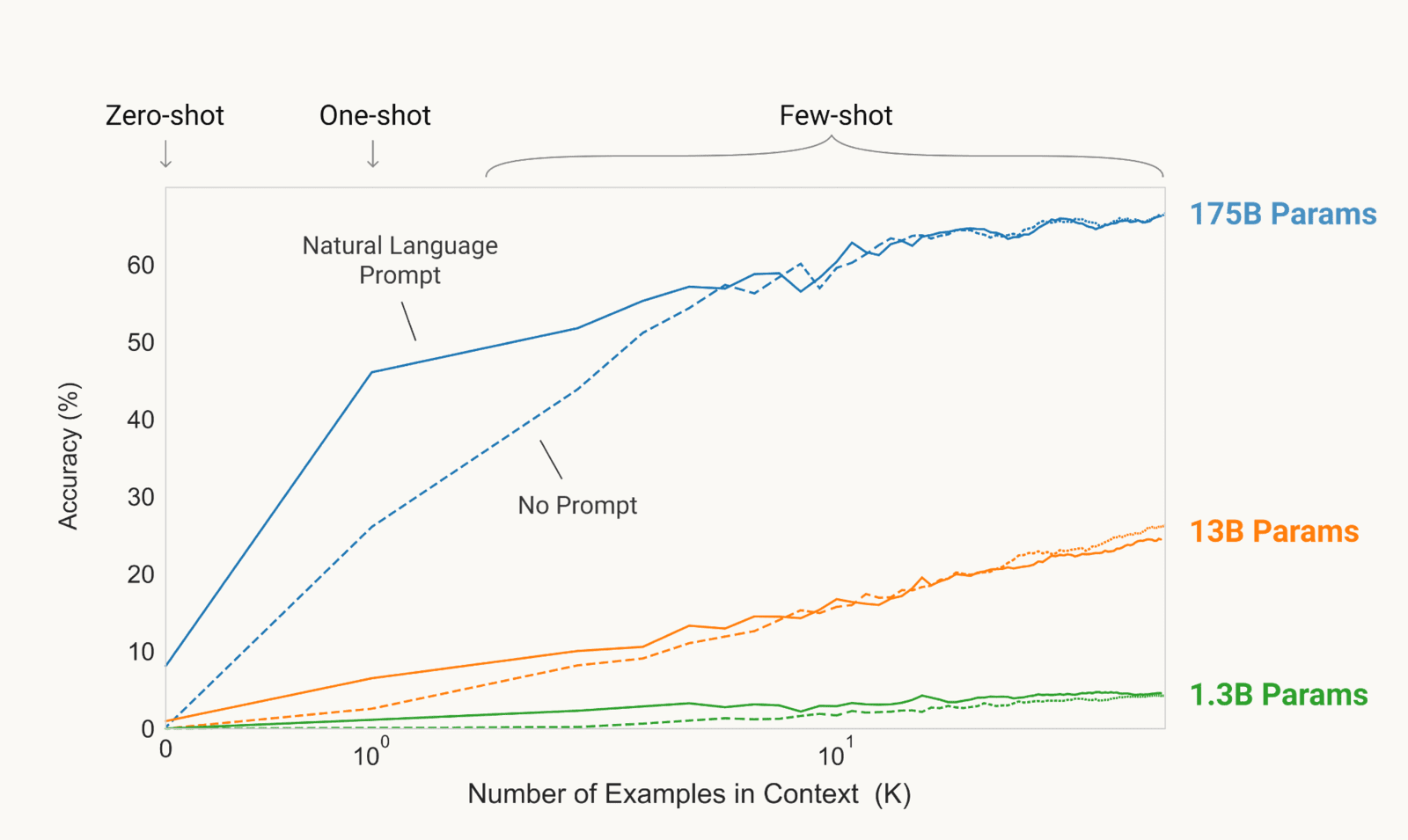
Published figure from Brown et al. (2020), the GPT-3 paper, showing accuracy on a word-unscrambling task against the number of examples placed in the prompt. The horizontal axis is the number of examples in context, 0 at the left, then 1 and 10 on a logarithmic scale; labels above mark zero-shot (no examples), one-shot (one example) and few-shot (many). The vertical axis is accuracy in percent, 0 to about 67. Three colored groups of lines are labeled 175B, 13B and 1.3B parameters; for each size a solid line is a prompt that also describes the task in natural language and a dashed line has no such description. The 175-billion-parameter model starts at about 8 percent with no examples, reaches about 46 percent with one example when the task is described (about 26 without), and climbs to about 67 percent. The 13-billion model rises from about 1 to about 25 percent, and the 1.3-billion model stays below 5 percent. The task description helps mostly when examples are few. The slide uses the figure to show that in-context learning improves with model size and with more examples.
Open full-size figureIn the figure: solid = prompt opens with a one-sentence instruction ("Please unscramble the letters…"); dashed "No Prompt" = examples only, no instruction
- Published result, GPT-3 on the task of the previous slide: accuracy grows with the number of examples and with model size. No weight changes. Next: our replication with GPT-2
Slide 16
Our replication: in-context learning in GPT-2
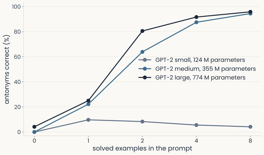
Real computation on three small public models, GPT-2 small (124 million parameters), medium (355 million) and large (774 million). A line plot with solid points joined by lines. The horizontal axis is the number of solved examples in the prompt, at 0, 1, 2, 4 and 8. The vertical axis is the percentage of antonym questions answered correctly, 0 to 100. The prompt is a list of word pairs such as hot, cold, followed by a new word whose opposite the model must produce. GPT-2 small stays low at every count, peaking at about 10 percent with one example and sliding to about 4 percent at eight. GPT-2 medium rises from 0 to about 22, 64, 88 and 94 percent. GPT-2 large rises from about 4 to 25, 81, 92 and 96 percent. The two larger models nearly coincide by eight examples. No weights change in any of these runs; only the prompt grows. The slide uses this to show that in-context learning appears with scale and improves with examples, using models students can run themselves.
Open full-size figureComputed for this course: GPT-2 small, medium and large, weights as trained · antonym task · 32 pairs, 24 test words × 3 random orders per point
- Prompt:
hot -> cold,big -> small, …wet ->. 8 examples: medium and large 94–96%, small < 10%; 0 examples: all ≈ 0 → the examples define the task; only the larger models use them
Slide 17
In-context learning: surprising results
Beyond accuracy curves: what does the model take from the examples?
- A new language from one book: Kalamang (< 200 speakers, almost no web text). With a grammar book in its prompt, Gemini 1.5 translates English → Kalamang about as well as a person who learned from the same book
- Wrong labels in the examples (task: is a movie review positive or negative?):
- Random labels on the examples: accuracy barely drops → the examples mostly show the format and the possible answers
- Flipped labels (positive reviews labeled "negative" and vice versa): large models flip their answers too, following the prompt over what they learned in pretraining; small models keep answering correctly
- More examples keep helping: with long contexts, hundreds to thousands of examples (many-shot) → further gains
Slide 18
Where in-context learning comes from
Nobody trained for this ability: where does it come from?
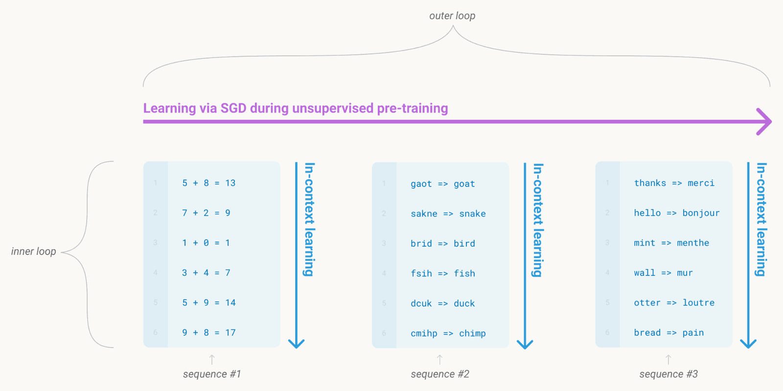
Published diagram: Figure 1.1 of Brown et al. (2020), the GPT-3 paper, a schematic of language-model meta-learning with two nested loops. The outer loop is learning by stochastic gradient descent during pretraining, which runs over many text sequences. Inside each sequence is an inner loop of in-context learning, a list of examples of one task followed by a new case the model must complete. Three example sequences are shown: addition, such as 5 + 8 = 13 and 7 + 2 = 9, then a new sum; unscrambling words, such as gaot => goat, then a new scrambled word; and translating English to French, such as thanks => merci, then a new word. The point is that the model learns, across training, to pick up a task from the examples in its own context. The slide uses this to name in-context learning as a skill acquired by pretraining on text, with no weight update at test time.
Open full-size figure- GPT-3's account: pretraining contains two nested loops (figure), one that changes the weights and one that does not → next slide
Slide 19
Two loops during pretraining
Ordinary next-token training, described as two loops:
- Outer loop: gradient descent across millions of documents; the weights change
- Inner loop: within one document, e.g.
hot → cold · big → small · wet →. Fromwet →alone,dryis a guess; using the two examples before it, it is easy. No weight changes, only the context grows - The loss scores every token,
dryincluded, and documents like this are everywhere on the web → gradient descent favors weights that use the examples: meta-learning - Your prompt is a new document: at use time, only the inner loop runs
Slide 20
Mechanism 1 (last lecture): induction heads copy
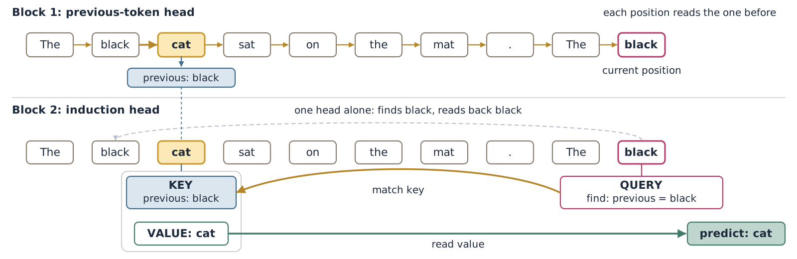
Diagram drawn for this lecture: how two attention heads in two successive blocks of a transformer predict the next word of The black cat sat on the mat. The black. Two horizontal bands each show the same ten tokens as boxes, with the last token, black, marked as the current position. The top band, block 1, is a previous-token head: each position reads the token before it, and the first cat receives a tag reading previous: black. The bottom band, block 2, is an induction head. The last black issues a query, find: previous = black. This query matches the key on the first cat, previous: black, along a curved gold arrow. The value on that cat, cat, is read and goes to a box reading predict: cat. A faint dashed arrow from the last black back to the first black is labeled one head alone: finds black, reads back black. It shows what one head alone would do: it finds the earlier black and returns black. The slide uses this to show that an induction head copies the word that came after an earlier occurrence of the current word, and that it needs the tag written by the previous-token head in the block before.
Open full-size figure- Previous-token head tags each token with the one before; at the second black, the induction head finds the token tagged "previous: black" → copies cat. Forms abruptly in training, when in-context learning jumps (Olsson et al.)
Slide 21
Mechanism 2: heads that encode the task
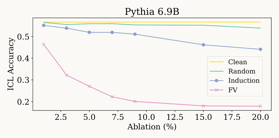
Published figure: Figure 1a of Yin and Steinhardt (2025), Which attention heads matter for in-context learning?, ICML 2025. A line plot titled Pythia 6.9B. The horizontal axis is ablation, the percentage of the model's attention heads that are knocked out, from 1 to 20 percent. The vertical axis is in-context learning accuracy on few-shot tasks, from about 0.15 to 0.6. Four lines are drawn. Clean, in yellow, is the intact model and stays flat at about 0.56. Random, in green, knocks out randomly chosen heads and stays near 0.55, ending at about 0.54 at 20 percent. Induction, in blue with round markers, knocks out induction heads. Accuracy falls slowly, from about 0.55 at 1 percent to about 0.44 at 20 percent. FV, in pink with crosses, knocks out function-vector heads. Accuracy falls quickly, from about 0.46 at 1 percent to about 0.32 at 3 percent, about 0.20 at 9 percent and about 0.18 at 15 and 20 percent. The slide uses this to show that function-vector heads matter much more for learning a task from examples than induction heads do.
Open full-size figureIn the figure: ICL = in-context learning · FV = function-vector heads · ablation = knockout
- Function-vector heads: a few heads, the same for every task, whose output vector encodes which task the examples show (antonym, capital of, …)
- Knock out FV heads → few-shot accuracy falls to about a third; knock out induction heads → it drops only a little. Copying ≠ learning a task from examples (12 models, up to 6.9 B parameters)
Slide 22
Mechanism 3: learning without backprop
Third account: can a forward pass itself carry out a learning algorithm?
- In-context learning is learning without backprop: the forward pass itself does the fitting
- Test case: put pairs (x, y) from a line in the prompt, then a new x → the transformer predicts y as least squares or ridge regression would
- How: one attention layer (without softmax) can carry out one gradient-descent step on the examples in its prompt; the weights never change
Slide 23
The same recipe in real systems
What a 2026 model is, and what every prompt does
Slide 24
From GPT-2 to today's assistants
Same recipe, GPT-2 to today: what changed?
- 2019, GPT-2: writes fluent paragraphs from a prompt
- 2020, GPT-3: learns new tasks from a few examples in its prompt
- 2022, ChatGPT: GPT-3.5 trained further to follow instructions and hold a conversation (next slides)
- 2023 on, frontier assistants: OpenAI GPT-4 and GPT-5, Anthropic Claude, Google Gemini (closed); Meta Llama, DeepSeek, Alibaba Qwen (open weights)
- 2024–25, reasoning models (OpenAI o1, DeepSeek-R1): write out steps before answering (see Reasoning, below)
- The core has not changed since GPT-2: a transformer pretrained to predict the next token; what changed is the scale and the training that comes after
Slide 25
From autocomplete to assistant
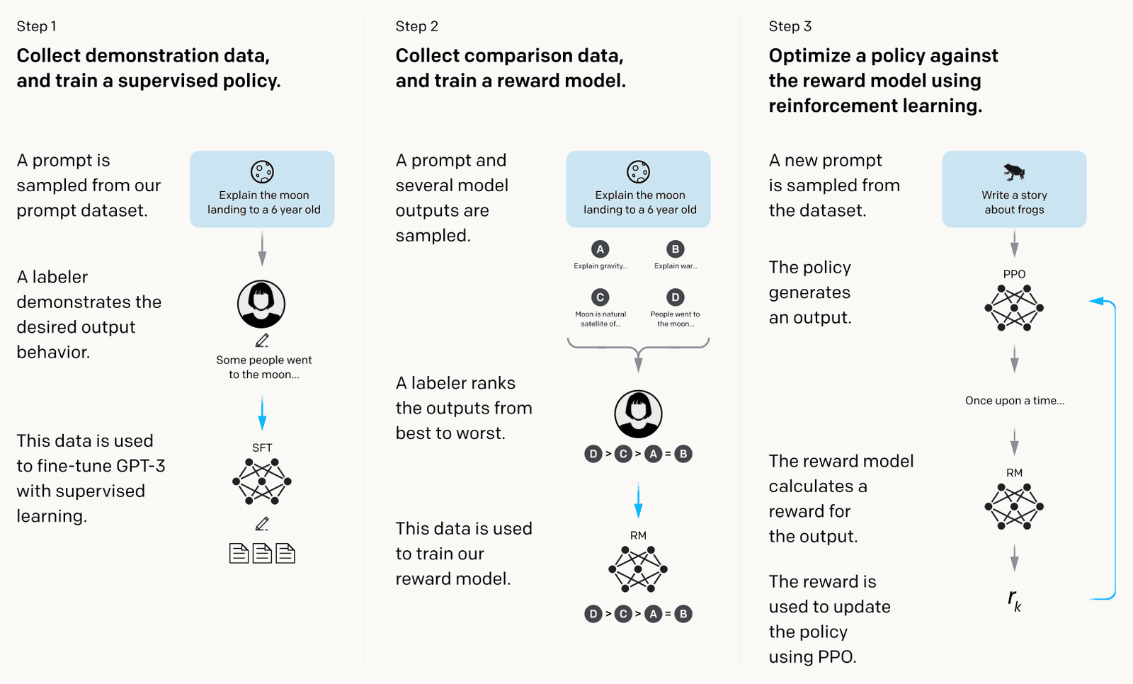
Published diagram: Figure 2 of Ouyang et al. (2022), the InstructGPT paper, showing three training steps as three panels from left to right. Step 1, supervised fine-tuning: a prompt such as Explain the moon landing to a 6 year old is given to a human labeler, who writes a good answer; GPT-3 is fine-tuned on these demonstrations. Step 2, reward model: the model writes several answers to a prompt, a labeler ranks them from best to worst, and the rankings train a reward model that scores answers. Step 3, reinforcement learning: for a new prompt such as Write a story about frogs, the model writes an answer, the reward model scores it, and that score updates the model with a policy-gradient method (PPO). Arrows connect prompts, outputs, labelers and models. The slide uses it to show how a pretrained next-token predictor becomes an assistant that follows instructions.
Open full-size figure- RLHF (reinforcement learning from human feedback), InstructGPT's recipe: SFT (supervised fine-tuning) on demonstrations → reward model fit to human rankings → PPO against it
Slide 26
After InstructGPT: simpler and checkable rewards
RLHF is costly: later post-training drops the reward model, then the human labels.
- DPO (direct preference optimization): learns from the same human choices between two answers, with no reward model and no reinforcement-learning loop
- Reinforcement learning from verifiable rewards: reward answers a program can check (a math result, code that passes its tests) → no human labels needed → reasoning models (next slides)
- All these stages keep training the same pretrained network: post-training
Slide 27
Writing an answer is choosing a path
Why would writing out steps help a model answer?
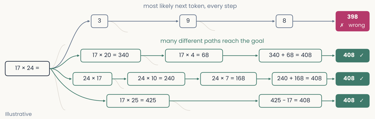
Diagram drawn for this lecture, labeled Illustrative: a tree of token choices for the prompt 17 times 24 equals. The prompt is a box at the left. Four paths leave it, each a row of boxes joined by arrows and ending in a box at the right. The top path, labeled most likely next token, every step, takes the single most likely token each time: 3, then 9, then 8. It ends in a magenta box, 398, marked wrong. The three paths below, labeled many different paths reach the goal, write intermediate steps in green boxes. The first reads 17 times 20 = 340, then 17 times 4 = 68, then 340 + 68 = 408. The second reads 24 times 17, then 24 times 10 = 240, then 24 times 7 = 168, then 240 + 168 = 408. The third reads 17 times 25 = 425, then 425 - 17 = 408. All three end in a green box, 408, marked correct. Faint grey stubs branch off several boxes and stand for other continuations the model could have chosen. The probabilities of the choices are not from a real model. The slide uses this to show that an answer is a path through a large tree of continuations, and that choosing the most likely token at each step can end in a wrong answer.
Open full-size figure- An answer is a path through a huge tree of continuations: the most likely token at every step (greedy) can dead-end; many paths reach the goal
- Intermediate steps make the next ones easy → writing them out helps (next slide)
Slide 28
Reasoning: thinking in tokens
Two ways to get intermediate steps: prompt for them, or train for them.
- Chain of thought: worked solutions with intermediate steps in the prompt → large models write steps too and solve far more math word problems (8 examples: state of the art for a 540 B model)
- No examples needed: add "Let's think step by step" → large gains on arithmetic and logic tasks
- Reasoning models (OpenAI o1, DeepSeek-R1): reinforcement learning on answers a program can check, no human-written reasoning → step-by-step answers, self-checking and backtracking emerge
- More tokens = more computation per answer (test-time compute) → thinking longer helps on hard problems
Slide 29
Inside a 2026 model
Same pretrained core, seen from inside: how do models grow without cost growing with them?
- Mixture of experts: each block's MLP is split into many smaller MLPs, the "experts"; for each token, a learned router picks a few experts and only those run → DeepSeek-V3: 671 B parameters in total, 37 B used per token
- Multimodal: image patches as tokens → one transformer for text and images
- Long context, growing fast: GPT-3 (2020) 2 K tokens → GPT-4 Turbo (2023) 128 K → Gemini 1.5 (2024) 1 M → Llama 4 Scout (2025) 10 M, dozens of novels
- Hybrids: many long-context models replace most attention layers with recurrent ones, which are cheaper on long inputs (next lecture)
Slide 30
Every prompt is in-context learning
Back to the prompt: what does an assistant read before it answers?
- One long context: the provider's instructions, your earlier messages, any examples you give, and text the system adds for you, such as web pages, files and tool results. Adding retrieved text this way is retrieval-augmented generation
- The model draws on two sources. The weights hold what it learned in pretraining; the context holds what you and the system have written so far. Only the context changes during a conversation
- The weights do not learn from your conversation: when the context is gone, so is everything in it. Saved "memories" are text put back into a later context
- Long contexts are expensive: the KV cache (keys and values of every token, last lecture) must be stored → a 1 M-token window needs a lot of memory
Slide 31
Tools and agents
The context can also hold tool results: the model's text triggers actions.
- Two actors: the model only writes text; the system, an ordinary program around it, runs tools and pastes their results into the model's context
- Tool call: the model writes
search("Natural Stories reading times")→ the system runs the search → the results go into the context - Agent = model + system in a loop: the model writes code → the system runs it → the model reads the error and writes a fix → … until the task is done
- Everything the agent knows about your task sits in its growing context → it can lose track of a long task
Slide 32
A model of the reader, and of the brain?
Two tests of the same model: word probabilities → reading times and N400; internal activations → brain responses
Slide 33
Surprisal: how unexpected a word is
First test: do a model's word probabilities predict readers and the N400?
- Surprisal: how unexpected a word is given the words before it. 0 bits = certain; 10 bits ≈ a probability of 1/1,000. Same as the per-word training loss, in bits instead of nats
- Surprisal theory (psycholinguistics, before LLMs): reading time (how long readers spend on a word) grows ~linearly with surprisal
- N400 (opening sentence): larger for unexpected words → LLM surprisal predicts its size word by word
- An LLM gives the surprisal of every word in any text → both predictions can be tested at scale
Slide 34
Surprisal from a real model, token by token
What does surprisal look like from a real model?
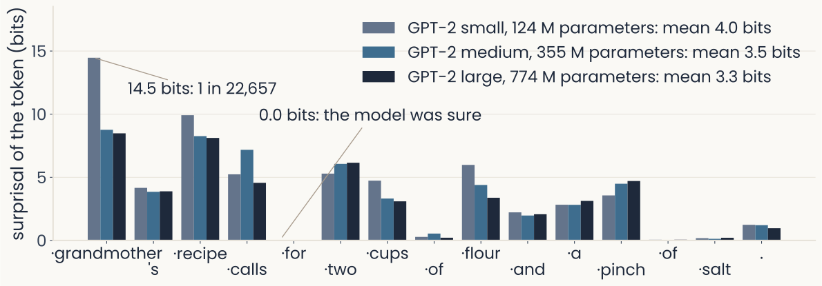
Real computation on three public models, GPT-2 small (124 million parameters), medium (355 million) and large (774 million). A grouped bar chart. The horizontal axis lists the tokens of the sentence My grandmother's recipe calls for two cups of flour and a pinch of salt, with a leading space marked by a dot; the first token has no bar because nothing precedes it. Each token has three bars, one per model, giving its surprisal in bits, the negative base-2 log probability the model gave it given the earlier words, on a vertical axis running 0 to about 15. Grandmother is the tallest, 14.5 bits for the small model (a callout says about 1 chance in 22,657) and about 8.5 for the medium and large ones. Recipe is about 8 to 10 bits. The token for and the second of are near zero, and a callout notes that 0 bits means the model was sure. Salt is also near zero. Mean surprisal over the sentence is 4.0, 3.5 and 3.3 bits for small, medium and large. The slide uses this to show what surprisal is and that bigger models are on average less surprised.
Open full-size figureReal computation: GPT-2 small, medium and large, weights as trained · a dot marks a token that begins with a space
- Each bar is of the probability the model gave the token that actually came next. Function words (small grammar words: for, of, a) cost almost nothing; the first content word (noun, verb, adjective), grandmother, costs 14.5 bits. Bigger model, fewer bits: 4.0 → 3.5 → 3.3 on average
Slide 35
What it means to predict reading times
From per-word surprisal to a test against readers' behavior.
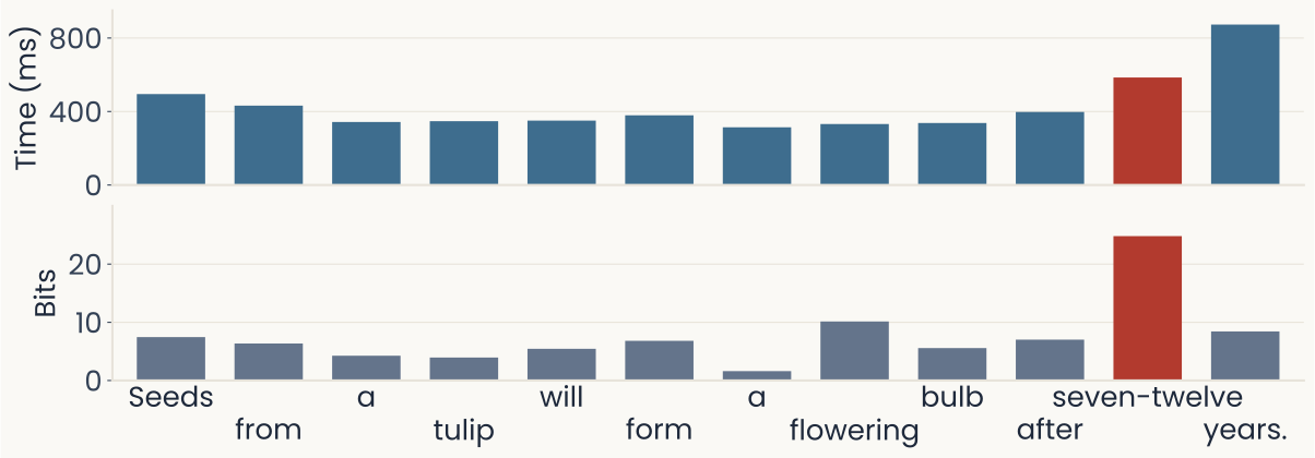
Real data and computation on one sentence from the Natural Stories self-paced reading corpus, Seeds from a tulip will form a flowering bulb after seven-twelve years. Two stacked bar charts share the same twelve words along the bottom. The top chart gives mean reading time in milliseconds, 0 to about 900, averaged over many readers. Most words sit between about 310 and 500 ms (Seeds about 490, a about 310). Seven-twelve, drawn in red, is about 580 ms, and the final word years is the slowest at about 870 ms. The bottom chart gives each word's surprisal in bits under GPT-2 small, 0 to about 25. Most words are 2 to 10 bits (flowering about 10, the second a about 2), while seven-twelve, also in red, is the clear peak at about 25 bits. The unexpected word draws the highest surprisal and a longer reading time, and the slowdown carries into the next word. The slide uses this to link model surprisal to human reading times.
Open full-size figureReal computation: Natural Stories self-paced reading times · GPT-2 small surprisal, whole story as context
- Self-paced reading: readers press a key to reveal each word. The unexpected seven-twelve (24.8 bits) slows them down, and the slowdown spills onto the next word. Next: the whole story
Slide 36
Reading time against surprisal, the whole story
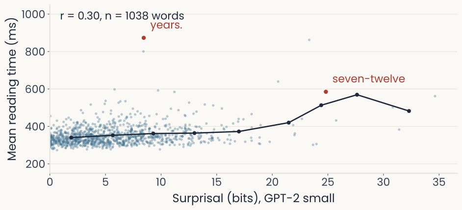
Real data and computation on one story of the Natural Stories self-paced reading corpus. A scatter plot with one dot for each of the 1,038 words of the story. The horizontal axis is the word's surprisal in bits under GPT-2 small, with the whole story as context, from 0 to about 35. The vertical axis is the mean reading time of the word in milliseconds, averaged over readers, from 200 to about 1,000. Most dots are blue and pale, and they pile up at surprisal below 15 bits and reading times between about 300 and 450 ms. A dark line joins the means of the dots in successive surprisal bins. It rises slowly from about 340 ms near 2 bits to about 370 ms near 17 bits, then climbs to about 570 ms near 28 bits, and ends lower, at about 480 ms near 32 bits, where few words fall. Two words are drawn in red. Seven-twelve is at 24.8 bits and about 585 ms. Years is at 8.4 bits and about 873 ms, far above the line for its surprisal. Text in the corner reads r = 0.30, n = 1038 words. The slide uses this to show that more surprising words are read more slowly, with a lot of scatter, and that surprisal explains about 9 percent of the variance in reading time.
Open full-size figureReal computation: Natural Stories, one story · GPT-2 small, whole story as context · dot = one word · line = mean per bin
- More surprising words are read more slowly, r = 0.30, with a lot of scatter: surprisal explains ~9% of the variance. Next: what surprisal adds beyond word length and frequency
Slide 37
Against human readers: bigger is not better
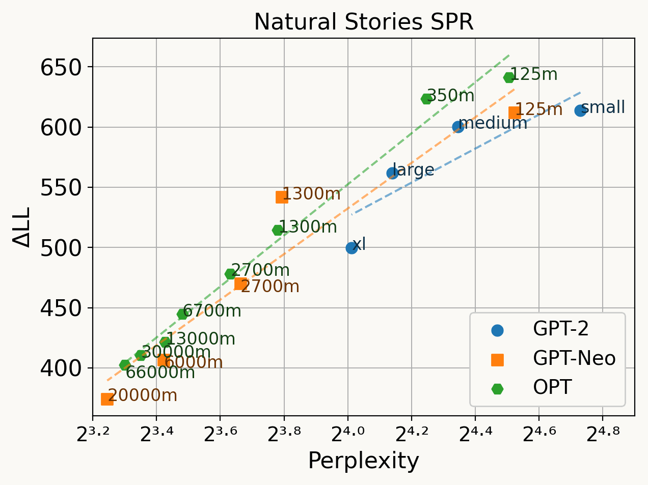
Published figure: Figure 1 of Oh and Schuler (2023), panel for the Natural Stories self-paced reading corpus. A scatter plot. The horizontal axis is language-model perplexity on a log scale, from about 2 to the 3.2 to 2 to the 4.8; the vertical axis is delta log-likelihood, the gain in how well a regression predicts human reading times when the model's surprisal is added, from about 375 to 640. Three model families are plotted with dashed least-squares lines: GPT-2 (blue circles, small to XL), GPT-Neo (orange squares, 125 million to 20 billion parameters) and OPT (green hexagons, 125 million to 66 billion). Each point is labeled with its size. In every family the smallest models, with the highest perplexity, give the largest gain, near 600 to 640, and the largest models give the smallest, near 380 to 400. Better next-word predictors therefore explain reading times worse. The slide uses this to show that the best language model is not the best model of human reading.
Open full-size figureEach dot = one model (label = size) · left = lower perplexity, better text prediction · up = better fit to reading times · in every family, bigger models sit lower
- ΔLL: gain in fit to reading times when surprisal is added to word length and frequency. Better text prediction → worse fit to readers, as better ImageNet models became worse models of IT
Slide 38
Try it: what did the model expect?
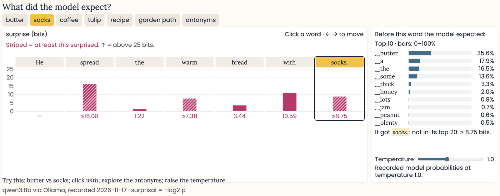
What did the model expect demo: the socks sentence with a surprisal bar per word; socks is outside the model's top 20 guesses, at least 8.75 bits. The side panel lists what the model expected after with: butter 36%, a 18%, the 17%, some
Open full-size figure- For you to try at home: a real 8 B model's surprisal for each word, and what it expected instead
Slide 39
Better language model, better brain model?
Reading times disagree with scale: what about brain responses?
- Brain responses: yes, so far. Models that predict the next word better also predict brain responses to language better. This holds in fMRI (blood oxygenation, whole brain, a few seconds' resolution) and ECoG (electrodes on the surface of the cortex, milliseconds), and the fit grows logarithmically with size up to 30-billion-parameter models
- Measured with an encoding model: a ridge readout from the model's activations to each voxel or electrode, as for IT
- Reading times: no, past a point. Surprisal from larger models fits readers worse (previous slide)
- Open: brain data and reading times disagree about the best model. Possible reason: a large model has read far more text than any person, so it finds words predictable that a reader does not
Slide 40
Using the model to control the brain
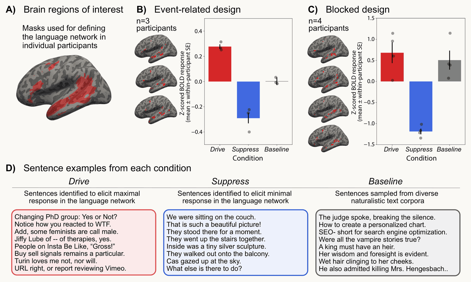
Published figure: Figure 2 of Tuckute et al. (2024), driving and suppressing the human language network with sentences chosen by a language model. Panel A shows the left hemisphere on an inflated brain, with the language network in red along the temporal lobe and in frontal cortex, defined separately for each participant. Panel B is a bar chart for an event-related design with three participants. Vertical axis: z-scored fMRI (BOLD) response of the language network; bars for the drive, suppress and baseline conditions. Drive sentences are highest at about 0.28, suppress sentences are lowest at about minus 0.29, and baseline is near 0; dots show individuals. Panel C is the same for a blocked design with four participants: drive about 0.7, suppress about minus 1.2, baseline about 0.5. Panel D lists example sentences. Drive sentences are odd or fragmentary, such as Jiffy Lube of -- of therapies, yes. Suppress sentences are plain, such as We were sitting on the couch. Baseline sentences are ordinary corpus text. The slide uses this to show that a model of language can predict, and control, activity in the brain's language regions.
Open full-size figure- Encoding model: GPT-2 XL → fMRI of the language network (areas more active for sentences than nonwords). It then picks new sentences to raise or lower the network's response → confirmed in new participants
Slide 41
The brain as a prediction machine
- Predictive coding: the brain runs an internal generative model, predicts its input, and passes up only the prediction error, the part the prediction did not explain
- In language: surprisal tracks N400 size and reading time → consistent with prediction
- With GPT-2: adding the model's activations for the next ~8 words improves the fMRI fit → brain activity carries information about upcoming words
- Still a hypothesis: recordings across cortical layers show feedback that enhances predicted activity rather than cancelling it. Details in Going further
Slide 42
Open questions
- Brain or behavior? Which should a cognitive model answer to? Would a model trained on about as much text as a person reads fit both?
- Does the brain predict, or only carry information about what comes next? Brain activity that fits better when GPT-2 sees upcoming words shows that the brain holds information about the future. It does not show that the brain sends prediction errors up, as predictive coding says
- In-context learning in a brain? A model learns a task from its prompt with frozen weights, in its activations. Is some fast human learning also held in activity rather than in changed synapses? → Next lecture: recurrent networks, which also hold context in activity
Slide 43
Recap
- An LLM is a decoder transformer trained to predict the next token (word pieces from byte-pair encoding) on a very large amount of text
- In-context learning emerges from next-token training (no separate objective): GPT-2 medium and large show it, every prompt uses it, weights stay fixed
- Surprisal in bits, , from LLMs tracks brain responses, the N400 and reading times, but larger models fit readers worse while fitting the brain better, and a brain fit needs its controls
- Predictive coding: the brain may predict its input and send errors up; the evidence runs both ways
Slide 44
The assistant you may use on the project
- The AI assistants you may use on the project are the models from today
- They are trained to produce likely text, which is not always true text. So they hallucinate: they invent citations and results that look plausible. They are also prompt-sensitive: rephrase a question and the answer can change
- Contamination: public test questions end up in the training text → a model can answer them from memory, so a high benchmark score can overstate its ability. Testing an LLM in your project? Use items it cannot have seen
- So check every claim and citation an assistant gives you against its source; the writer–critic workflow from recitation does this systematically
Slide 45
For your final project
- Dates: teams registered on Canvas Thu 11/19 · proposal, one page per team, Sun 12/6 at 11:59 PM (moved from Wed 12/2) · poster session and report Mon 12/21 at 9:00 AM
- Data and models: anything from the lectures and assignments, or anything else you can get your hands on; GPT-2 or Pythia for surprisal run on the course Colab
- AI tools: allowed on the project, with disclosure; at the poster, either of you may be asked about any line of your code
- The brief, with dates and the proposal checklist: serre-lab.github.io/CPSY1291-2026/final-project
- Questions from today: which model size fits readers best, and does the answer change with the reading-time corpus?
- Exam 2: in class, Tue 12/1, Lectures 9–19; one sheet of notes, both sides
Slide 46
Further reading
Papers from today worth reading, for your project or out of interest.
- Oh & Linzen TICS 2026: to model human prediction, make language models less superhuman
- Hadidi et al. Nat Commun 2026: how model–brain alignment can arise from confounds
- Cai et al. Nature 2026: single human neurons during speech, read through a language model
- Goldstein et al. Nat Hum Behav 2025: one speech model's levels match the cortical hierarchy during real conversation
- AlKhamissi et al. EMNLP 2025: brain alignment tracks a model's grammar, not its world knowledge
- Westerberg & Roelfsema TICS 2026: cortical feedback during perception does not do what predictive coding predicts
Slide 47
Minute paper
Submit on Canvas → Minute papers → Minute Paper 18 (access code read out in class).
Write three brief points in your own words:
- A model answers a new task correctly after reading three solved examples in its prompt. What changed inside the model, and what did not? How is this different from fine-tuning?
- Something you do not yet understand, or a question still open
- Another idea you found interesting, and why it matters for brains, behavior or AI
Credit for a thoughtful attempt, not for being correct.
Slide 48
Going further
Predictive coding in detail
Slide 49
Language models and the brain: current readings
More encoding-model results, from conversation to single neurons, with a caution.
- Hours of real conversation: one speech-to-text model's sound, speech and word embeddings each predict ECoG activity across 100 h of everyday conversation, and the model's levels line up with the cortical hierarchy (Goldstein et al. 2025)
- Single neurons: the same readout, neuron by neuron, separates cells that track a word's part of speech and syntactic dependencies from cells that track phrase and sentence structure (Cai et al. 2026)
- What the fit tracks: across 34 saved stages of one training run, it follows a model's grammatical knowledge, not its world knowledge or reasoning (AlKhamissi et al. 2025)
- A caution from 2026: an untrained network, which has learned no language, can reach a good brain fit through shuffled train–test splits and confounds such as word rate (words per second). Some influential results were inflated this way (Hadidi et al. 2026)
Slide 50
Testing it with a language model
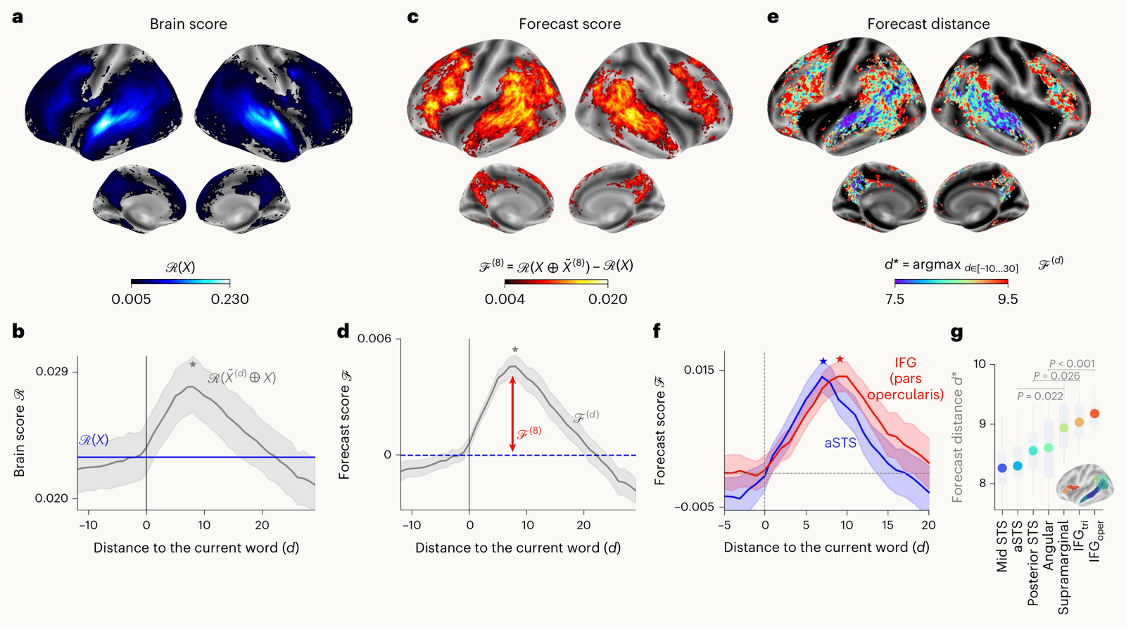
Published figure: Figure 2 of Caucheteux, Gramfort and King (2023), evidence for predictive coding in the brain during language comprehension. Seven panels labeled a to g, from fMRI of 304 people listening to stories. Panel a, brain maps: the brain score of GPT-2 activations, how well they predict each region's activity, from 0.005 to 0.230, is highest along the superior temporal sulcus. Panels b and d, line plots: adding the model's representation of the word d positions ahead (horizontal axis, distance to the current word, minus 10 to 30) raises the brain score, peaking at about 8 words ahead. Panel c, brain map: the regions where this forecast gain is significant, across temporal, parietal and frontal cortex. Panel e, brain map: the best forecast distance in each region, from 7.5 to 9.5 words. Panel f, line plots comparing two regions: forecast score peaks earlier in anterior superior temporal sulcus (about 7 words) than in inferior frontal gyrus (about 9). Panel g, dots by region, show best forecast distance growing from about 8 in the mid superior temporal sulcus to about 9.2 in frontal regions. The slide uses this to show that the brain appears to predict upcoming words, further ahead in higher regions.
Open full-size figure- 304 people heard stories in fMRI. Adding GPT-2's activations for the next 8 words improved the fit: brain activity carries information about upcoming words (prediction, or context? see Open questions)
Slide 51
Predictive coding and autoencoders
If the brain minimizes prediction error, how does that compare with an autoencoder?
- Autoencoder: minimizes the reconstruction residual by backprop (one forward, one backward sweep)
- Predictive coding minimizes the same residual by iterative settling (update until the error is small): a higher level's estimate of the causes relaxes until its prediction explains the input (Rao & Ballard 1999); the weights follow a local rule (each weight changes using only the activity of the two units it connects)
- Same residual, different algorithm: predictive coding needs only local error circuits, which may be how cortex does it
Slide 52
Rao & Ballard (1999)
- Each level predicts the level below through top-down connections; the residual, the prediction error, is sent bottom-up
- A higher level holds an estimate of the causes, predicts lower activity , and the error drives the update
- Trained on natural-image patches, it develops oriented, Gabor-like receptive fields, as sparse coding did, and predicts surround suppression (weaker response when the surround continues the pattern in the receptive field)
Slide 53
The predictive-coding equations
At one level: prediction of the level below , error .
Inference (fast, within one stimulus: settle to reduce the error):
Learning (slow, across stimuli: a local, Hebbian-like rule):
- is the top-down prediction; carries the error bottom-up
- Each update uses only quantities available at that connection, the error and the activity, so there is no global backward pass
Slide 54
Predictive coding as a deep net: PredNet
- Lotter, Kreiman & Cox stacked Rao–Ballard-style modules: each layer predicts the layer below and passes the prediction error up, trained on video to predict the next frame
- The trained network reproduces perceptual effects nobody built in, such as the flash-lag illusion
- From brain to AI: a 1999 theory becomes a trainable architecture
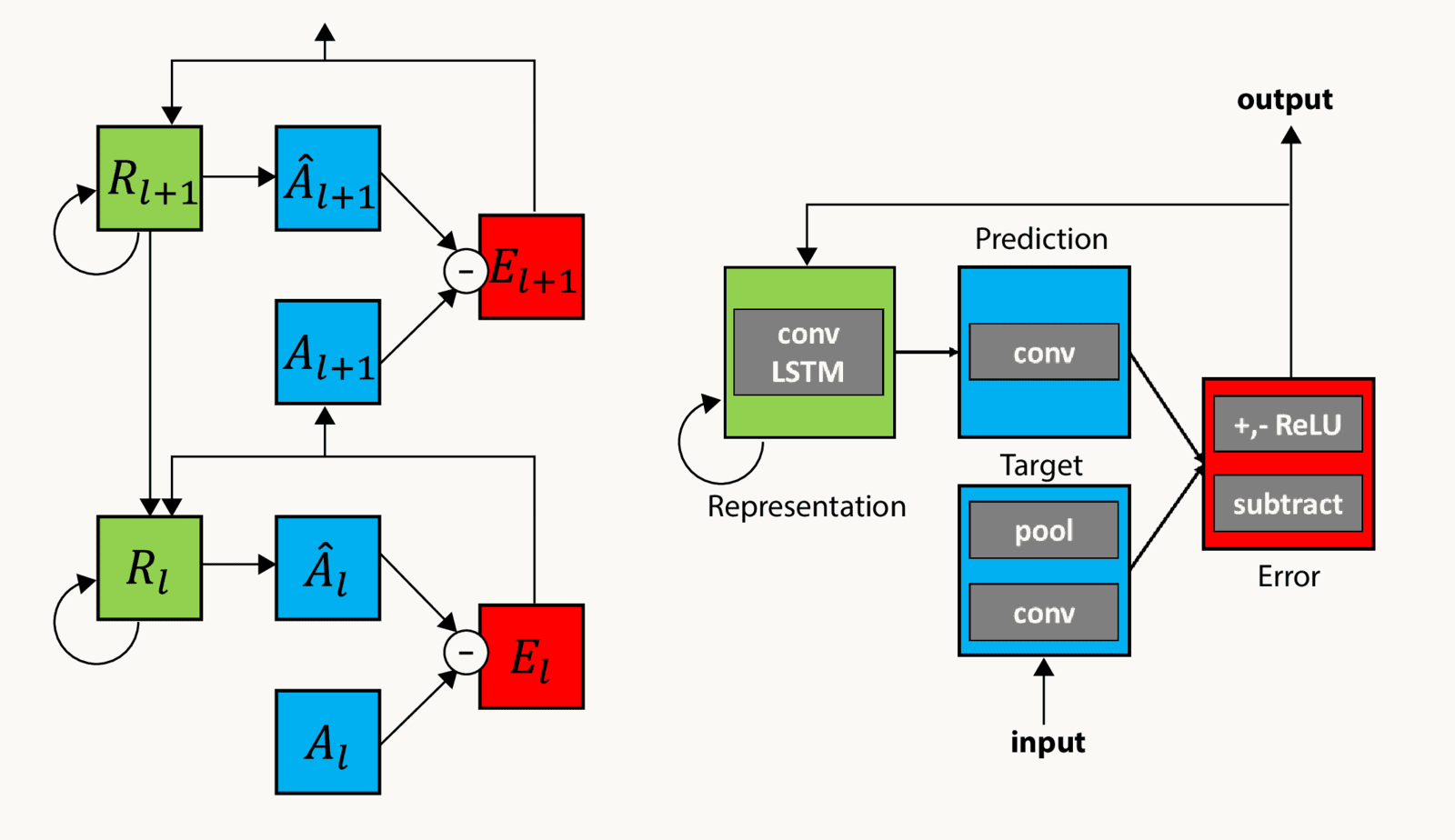
Published diagram: Figure 1 of Lotter, Kreiman and Cox (2016), the PredNet architecture. Left side: two stacked layers, l and l plus 1. Each layer has four kinds of square module. Green representation units R, with a recurrent loop arrow, send a prediction down to a blue module (A-hat), the predicted input. This is compared, through a circled minus sign, with a blue target module A, the actual input of that layer. The difference feeds a red error module E. Error signals go up the hierarchy to the next layer's target and to the representation units, and the representation of the higher layer passes downward to the one below. Right side: the same unit drawn with its operations. Representation is a convolutional LSTM; the prediction is a convolution; the target is a convolution then pooling of the input; and the error subtracts the two and applies a rectifier to the positive and negative parts. The slide uses this to show a network built around predicting its input and passing on only the error.
Open full-size figureSlide 55
Is backprop biologically plausible?
- Backprop's problems for biology: a separate backward pathway; weight transport (backward weights must equal the forward ones); a global two-phase schedule; non-local error signals
- Predictive coding offers local learning: errors computed in place by error units; updates use only the activity of the connected units
- Under some conditions predictive coding approximates the backprop gradient
- Still a hypothesis: direct evidence for cortical error units is debated