Learning the weights: from neurons to gradient descent

Reader-friendly version of the 29 lecture slides: the lecture content in normal flow, with figure descriptions and data tables where the figure carries data. Open the presentation.

Slide 1

CPSY 1291 Computational Methods for Mind, Brain & Behavior

Lecture 8 · Theme 2: Learning representations

Learning the weights: from neurons to gradient descent

Thursday, October 8 · Fall 2026

Return to contents

Slide 2

You have been using model neurons all along

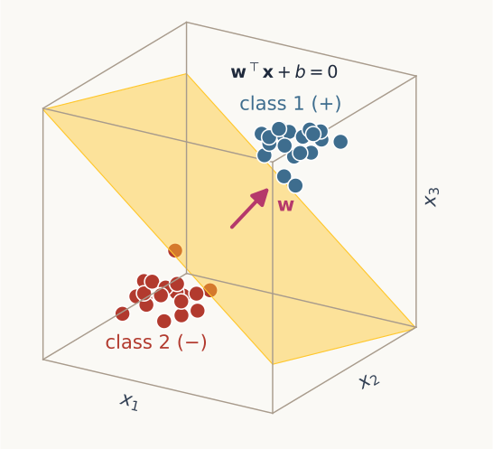
Two clouds of points in the space of three units x1, x2, x3, blue upper right and red lower left, separated by a gold hyperplane, the decision boundary, labelled w transpose x plus b equals 0; an arrow labelled w points from the plane toward the blue points

Open full-size figure

The readouts of the last lectures (animate or not, context, shattering, CCGP): a weighted sum of the responses, then a threshold: a decision boundary, a hyperplane in the space of units
The activations of the networks in the assignments: each number is one unit's output
Both are model neurons. Today: what one computes, how it relates to a real neuron, and how it learns its weights

Return to contents

Slide 5

What a real neuron does

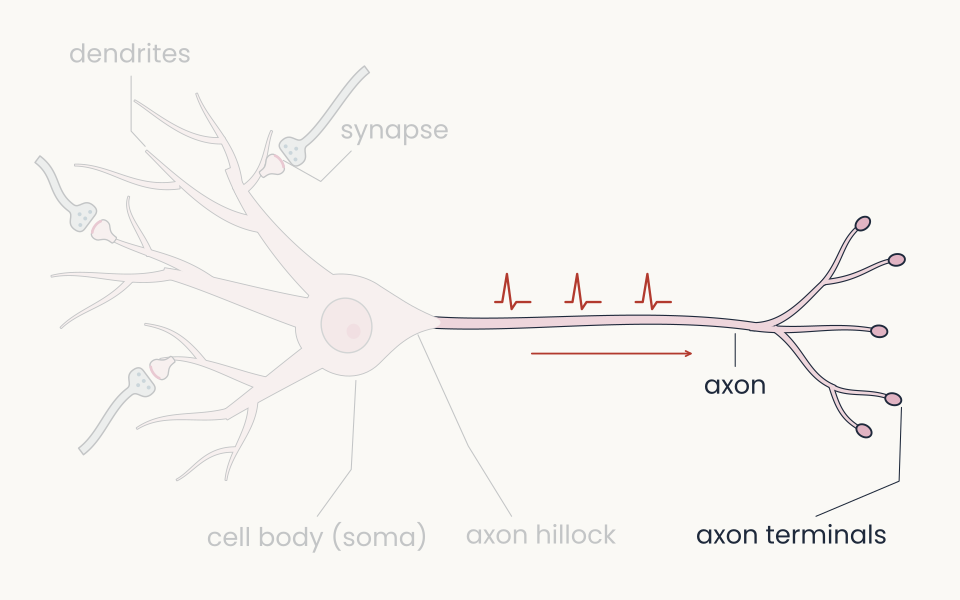
The same neuron drawing with the axon and the axon terminals highlighted and small spikes travelling along the axon to the right; the rest is faded
Open full-size figure

The dendrites collect inputs from other neurons: at each synapse, an incoming spike becomes a small electrical current
The cell body (soma) integrates them; past a threshold, the axon hillock fires a spike, a brief electrical pulse
The spike travels down the axon to the synaptic terminals: the inputs of the next neurons
Output: spikes; their number per second is the firing rate

London & Häusser Annu Rev Neurosci 2005 · Neuroscience background notes (PDF)

Return to contents

Slide 6

At a synapse: a spike becomes a current

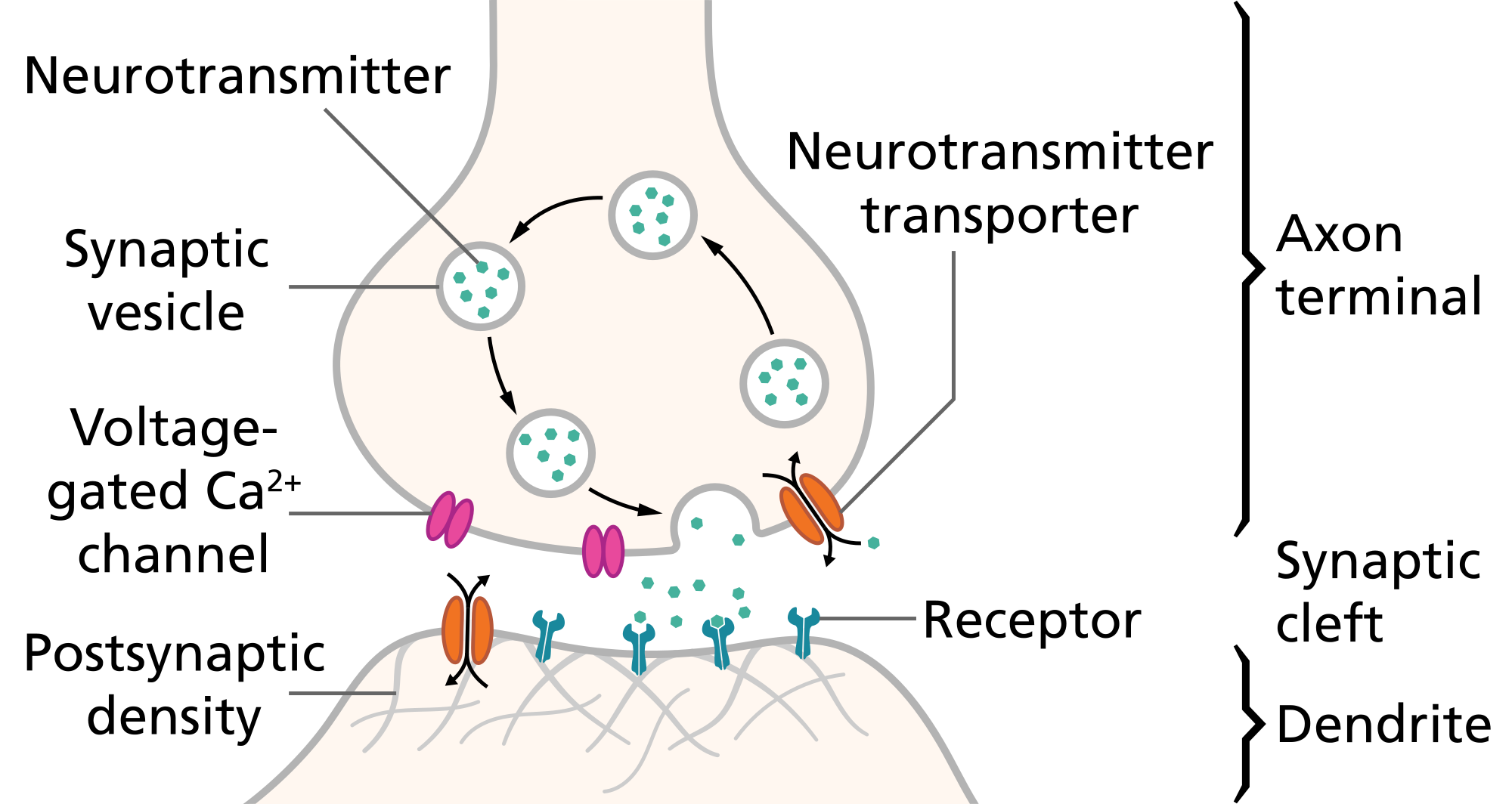
Schematic of a chemical synapse: the axon terminal of the presynaptic neuron holds vesicles filled with neurotransmitter; an arriving action potential opens voltage-gated calcium channels, vesicles fuse and release neurotransmitter into the synaptic cleft; it binds to receptors on the postsynaptic dendrite, which open and let ions flow in
Open full-size figure

A spike reaching the axon terminal releases neurotransmitter into the gap
It binds receptors on the next neuron, which open channels: ions flow in, a small current
Excitatory synapses push the neuron toward firing, inhibitory ones away; the currents of many synapses roughly add up at the soma
How much current one spike causes, the synaptic strength, is the main thing learning changes

Illustration: Thomas Splettstoesser CC BY-SA 4.0

Return to contents

Slide 8

From a neuron to a model neuron

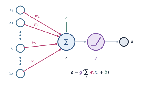
The model neuron: inputs x1 to xD, each with its weight w1 to wD, summed with a bias b into z, passed through the nonlinearity g, giving the output a = g(z)
Open full-size figure

Inputs $\textcolor{#3E6D8E}{x_i}$ : the firing rates of the neurons that connect to it
Weights $\textcolor{#B5396B}{w_i}$ : the strengths of those synapses, positive (excitatory) or negative (inhibitory) (minute paper)
Sum $z$ , with a bias $\textcolor{#3F7A6B}{b}$ : the currents adding up at the soma
Nonlinearity $\textcolor{#7A4FA3}{g}$ and output $a$ : the threshold at the axon hillock, and the firing rate
We drop spike timing, dendrites and chemistry: a point neuron

Return to contents

Slide 9

Building the neuron: inputs, weights and sum

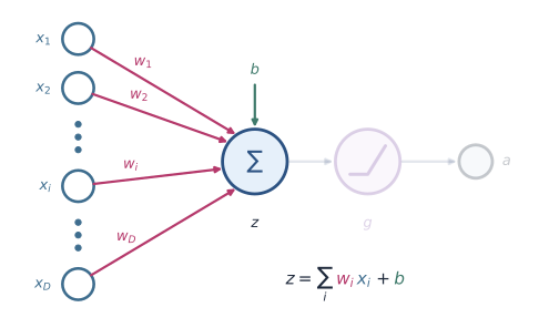
The complete model neuron with the inputs x1 to xD, their weights w1 to wD, the bias b and the summation node in full colour, and the nonlinearity g and the output a faded. The equation reads z equals the sum over i of w i x i plus b
Open full-size figure

Each of the $D$ inputs $\textcolor{#3E6D8E}{x_i}$ is a number: another neuron's output, or a stimulus feature such as a pixel
Each has a weight $\textcolor{#B5396B}{w_i}$ , positive (excitatory) or negative (inhibitory). Their sum, $z = \sum_i \textcolor{#B5396B}{w_i}\, \textcolor{#3E6D8E}{x_i} + \textcolor{#3F7A6B}{b}$ , is the pre-activation
Learning changes the weights and the bias. First we set them by hand

Return to contents

Slide 10

The weighted sum is a dot product

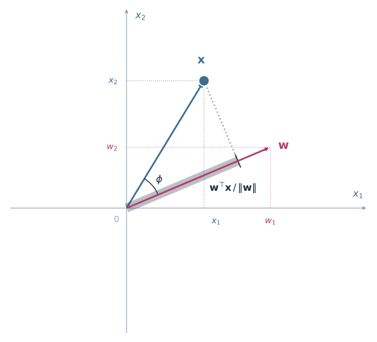
Axes x1 and x2. The input vector x in blue and the weight vector w in magenta, both from the origin, at an angle phi; a dark band along w marks the projection of x onto w, of length w transpose x over the length of w
Open full-size figure

Stack the inputs and weights into vectors $\textcolor{#3E6D8E}{\mathbf{x}},\,\textcolor{#B5396B}{\mathbf{w}}\in\mathbb{R}^{D}$ : the weighted sum is their dot product

z = \sum_{i=1}^{D} \textcolor{#B5396B}{w_i}\,\textcolor{#3E6D8E}{x_i} + \textcolor{#3F7A6B}{b} = \textcolor{#B5396B}{\mathbf{w}}^\top\textcolor{#3E6D8E}{\mathbf{x}} + \textcolor{#3F7A6B}{b}

Geometry (left): $\textcolor{#B5396B}{\mathbf{w}}^\top\textcolor{#3E6D8E}{\mathbf{x}} = \lVert\mathbf{w}\rVert\,\lVert\mathbf{x}\rVert\cos\phi$ , the length of the projection of $\textcolor{#3E6D8E}{\mathbf{x}}$ onto $\textcolor{#B5396B}{\mathbf{w}}$ , times $\lVert\mathbf{w}\rVert$
Aligned with $\textcolor{#B5396B}{\mathbf{w}}$ → large; perpendicular → zero; opposite → negative. The neuron asks how much of $\textcolor{#B5396B}{\mathbf{w}}$ is in the input

Return to contents

Slide 11

A neuron's weights set a decision boundary

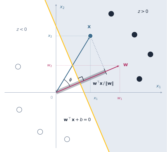
The same axes, w and x as on the previous slide, plus the decision boundary, the gold line where w transpose x plus b equals zero, perpendicular to w. The side where z is positive is shaded and holds filled dots; hollow dots lie on the other side. The projection of x onto w passes the line, so x falls on the positive side
Open full-size figure

The neuron computes $z = \textcolor{#B5396B}{\mathbf{w}}^\top\textcolor{#3E6D8E}{\mathbf{x}} + \textcolor{#3F7A6B}{b}$ ; its decision boundary is the line where $z = 0$
$\textcolor{#B5396B}{\mathbf{w}}$ is perpendicular to the boundary and points to the side where $z > 0$ ; $\textcolor{#3F7A6B}{b}$ slides the line without turning it
Add a threshold, and the neuron fires only on that side: one neuron is a linear classifier, the same readout that read context from the hypothetical three-neuron populations of the last two lectures (there, a plane in 3 units)
Every readout in this lecture is one model neuron

Return to contents

Slide 12

One weight vector, two readings

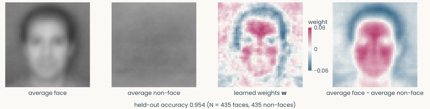
Four 48 by 48 pixel images in a row: the average face, the average non-face, the weights w of a readout trained to tell faces from other objects in Caltech-101 photographs, drawn with positive weights in magenta and negative in blue, and the average face minus the average non-face in the same colours. The weight image has a face-like layout of eyes, nose and mouth. Underneath, the readout's accuracy on held-out photographs

Open full-size figure

One neuron, one weight per pixel (2,304), trained to answer "face or not?"
As a boundary: it says "face" when $\textcolor{#B5396B}{\mathbf{w}}^\top\textcolor{#3E6D8E}{\mathbf{x}} + \textcolor{#3F7A6B}{b} > 0$ . As a template: drawn as an image, $\textcolor{#B5396B}{\mathbf{w}}$ has the layout of a face, and inputs that look like it give the largest $\textcolor{#B5396B}{\mathbf{w}}^\top\textcolor{#3E6D8E}{\mathbf{x}}$
Magenta weights push toward "face", blue toward "non-face". The weights best separate the classes; they are not the average face

Haufe et al. NeuroImage 2014 · Photographs: Caltech-101, Fei-Fei, Fergus & Perona 2004

Return to contents

Slide 13

A neuron is a feature detector: template matching

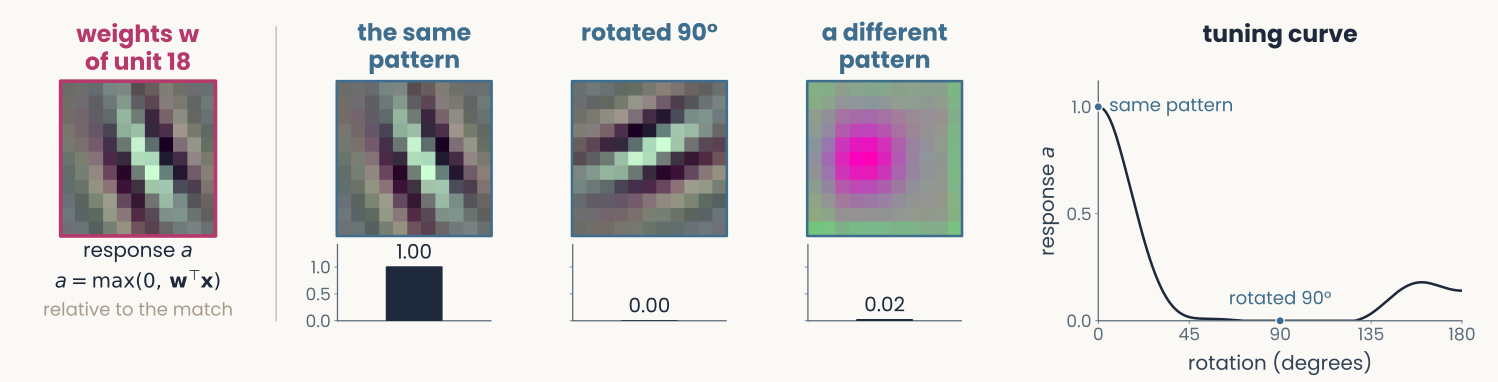
One unit of AlexNet's first layer: its weights shown as a small colour image of an oriented edge. Three inputs of the same length: the same pattern, the pattern rotated by 90 degrees, and a different pattern; under each, the unit's response relative to the first: 1.00 for the same pattern, 0.00 rotated, 0.02 for the different pattern. Right, the tuning curve: the response as the pattern is rotated from 0 to 180 degrees, 1 at 0 degrees, falling to 0 by about 45 degrees, 0 at 90, with a small bump near 160
Open full-size figure

A unit of the network you analyse in the assignments: its weights $\textcolor{#B5396B}{\mathbf{w}}$ , drawn as an image, look like the pattern it detects; rotating the input traces its tuning curve (right)
$\textcolor{#B5396B}{\mathbf{w}}$ and every input $\textcolor{#3E6D8E}{\mathbf{x}}$ have length 1, so $\textcolor{#B5396B}{\mathbf{w}}^\top\textcolor{#3E6D8E}{\mathbf{x}}$ is the cosine of their angle: 1 when $\textcolor{#3E6D8E}{\mathbf{x}}$ looks like $\textcolor{#B5396B}{\mathbf{w}}$ . The weights act as a template

Return to contents

Slide 14

Building the neuron: activation and output

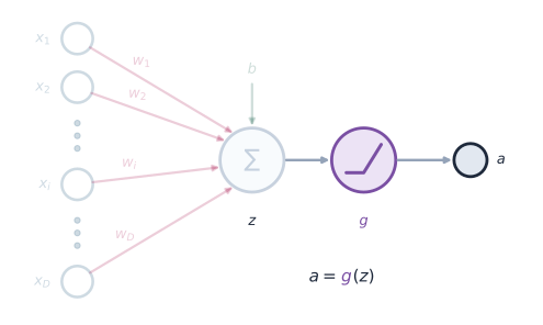
The same model neuron with the inputs, weights, bias and sum faded, and z, the nonlinearity g and the output a in full colour. The equation reads a equals g of z
Open full-size figure

$a = \textcolor{#7A4FA3}{g}(z)$ : the nonlinearity, most often ReLU, $\textcolor{#7A4FA3}{g}(z)=\max(0,z)$
The output $a$ is the neuron's activation, its stand-in for a firing rate
Why nonlinear? A real neuron fires nothing below threshold, then faster as its input grows

Glorot, Bordes & Bengio AISTATS 2011 (ReLU) · Nair & Hinton ICML 2010

Return to contents

Slide 15

Transfer functions: the nonlinearity $g$

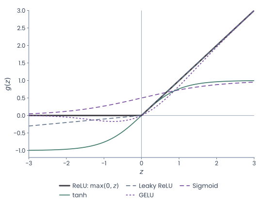
Five transfer-function curves on one set of axes: ReLU (thick), leaky ReLU, sigmoid, tanh and GELU
Open full-size figure

A real neuron's f–I curve (firing rate against input current): 0 below threshold, then rising, then saturating
History: a step (McCulloch & Pitts 1943, the perceptron), then sigmoid and tanh, smooth enough for backpropagation (1986), then ReLU (2010s), then GELU in transformers
None is exact: ReLU and GELU never saturate, the sigmoid never reaches 0, tanh, leaky ReLU and GELU give negative "rates"
ReLU (thick line) dominates: cheap, and deep networks train well with it

Return to contents

Slide 16

From weights set by hand to weights learned

The complete single neuron: weighted inputs summed with a bias into z, z passed through the nonlinearity g, giving the output a, labelled a = g(z)
Open full-size figure

So far we chose $\textcolor{#B5396B}{\mathbf{w}}$ and $\textcolor{#3F7A6B}{b}$ by hand. A cortical neuron has thousands of synapses, a network millions, even billions, of weights: the weights must be learned from examples
Learning needs a loss, one number that measures how wrong the outputs are, and gradient descent, which changes every weight to lower it
The nonlinearity $\textcolor{#7A4FA3}{g}$ sets the kind of output, each with its own loss: a threshold gives yes or no (perceptron), no nonlinearity ( $\textcolor{#7A4FA3}{g}(z)=z$ ) a number (linear regression), a sigmoid a probability (logistic regression), a softmax a probability per class

Return to contents

Slide 17

A network maps inputs to outputs

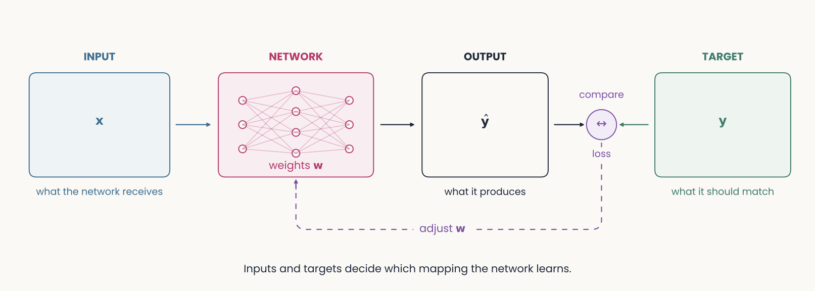
A diagram from left to right: an input x goes into a network drawn as layers of units with weights w, which produces an output y hat. The output is compared with a target y; the comparison gives the loss, and a dashed arrow labelled adjust w runs back into the network. Caption: inputs and targets decide which mapping the network learns

Open full-size figure

Training adjusts the weights so that, on many examples, the output matches the target. To train a network, choose inputs and targets

Return to contents

Slide 21

Where does the target come from?

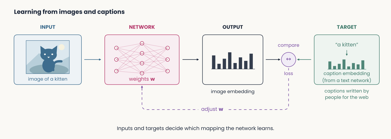
The same diagram for images and captions: the input is an image of a kitten, the output is an image embedding, and the target is the embedding of its caption, a kitten, computed by a text network; captions written by people for the web
Open full-size figure

Image → its caption, written by people for the web. An image network and a text network turn each into an embedding (a vector of numbers), and the two vectors are compared. The inputs and targets we choose decide which mapping the network learns

Brown et al. NeurIPS 2020 · Devlin et al. NAACL 2019 · Caron et al. ICCV 2021 · He et al. CVPR 2022 · Radford et al. ICML 2021

Return to contents

Slide 22

How can a readout learn its weights from labeled examples?

Return to contents

Slide 23

The first learning neuron: the perceptron

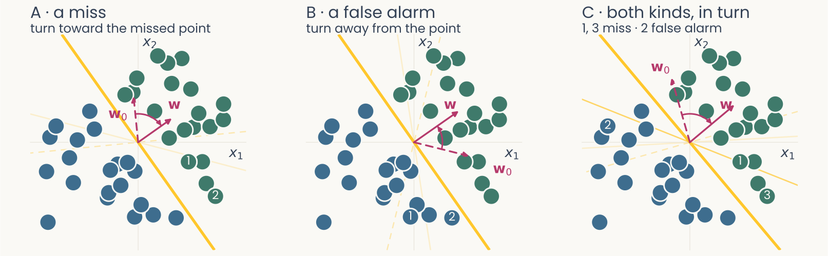
Three runs of the perceptron rule without a bias, on the same 2-D points separable by a line through the origin, each from a different starting weight vector. In each panel the decision line after every update is drawn from faint to dark, ending in a solid gold line that separates the classes, with the starting and final weight vectors as magenta arrows; under each panel, the mistakes per pass fall to zero
Open full-size figure

Rosenblatt (1958): a model neuron with a threshold that learns its weights from labeled examples, built in hardware
The rule is a heuristic: after a mistake, move $\textcolor{#B5396B}{\mathbf{w}}$ toward the missed example, or away from a false alarm. No loss lies behind it, yet if a line separates the classes, it stops (all three runs)
It learns from its mistakes: $\textcolor{#B5396B}{\mathbf{w}}$ changes only when the neuron is wrong

Rosenblatt Psychol Rev 1958 · Minsky & Papert Perceptrons, MIT Press 1969 · Perceptron notes (PDF), with worked examples

Return to contents

Slide 24

Which way is downhill? From derivative to gradient

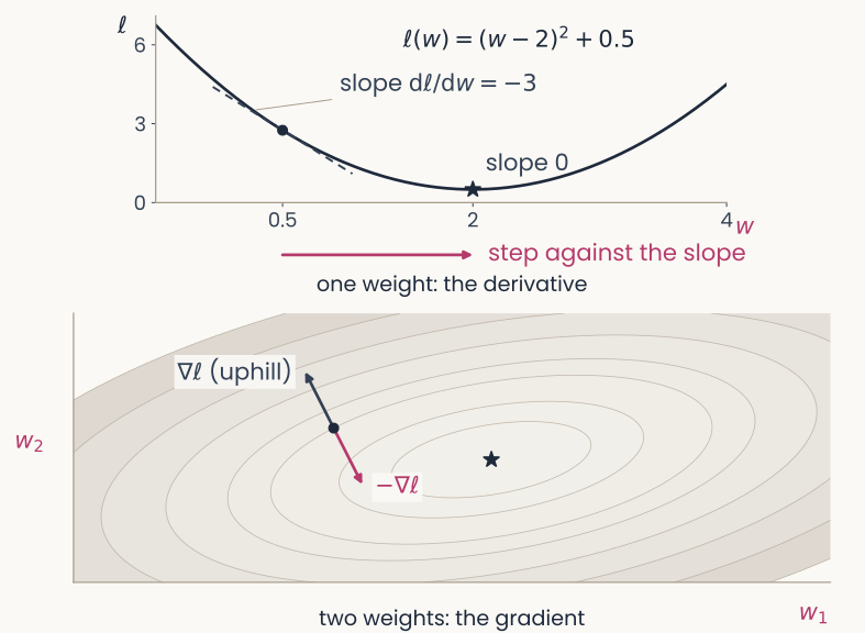
Two panels. Top, one weight: a U-shaped loss curve over w with a dot at w = 0.5, its tangent of slope minus 3, an arrow pointing toward the minimum, labelled step against the slope, and the minimum marked slope 0. Bottom, two weights: elliptical contours of the loss over w1 and w2 with the minimum marked; at a starting point, a gray arrow perpendicular to the contour labelled gradient, uphill, and a magenta arrow in the opposite direction labelled minus the gradient

Open full-size figure

The loss $\ell(\textcolor{#B5396B}{w})$ is a function of the weight: one number saying how wrong the outputs are
One weight: the derivative $d\ell/d\textcolor{#B5396B}{w}$ is its slope. Slope negative: increase $\textcolor{#B5396B}{w}$ ; positive: decrease it. At the minimum the slope is 0
Many weights: the gradient $\nabla\ell$ lists one slope per weight, $\partial\ell/\partial \textcolor{#B5396B}{w_i}$ : how fast $\ell$ grows when $\textcolor{#B5396B}{w_i}$ alone grows a little
The gradient points uphill. Gradient descent: a small step against it, $\textcolor{#B5396B}{\mathbf{w}} \leftarrow \textcolor{#B5396B}{\mathbf{w}} - \eta\,\nabla\ell$ , again and again; the learning rate $\eta$ sets the step size

Return to contents

Slide 25

The delta rule (Widrow–Hoff): step down a smooth error

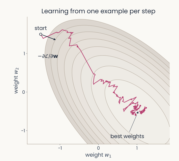
Contours of the loss for a two-weight linear regression, with the best weights marked by a star. From the start at the upper left, the path of the delta rule with a constant learning rate, one example per step, winds downhill toward the star; a short arrow at the start shows the direction minus the gradient

Open full-size figure

Widrow & Hoff (1960): write a loss and step down its slope. Drop the threshold so the loss is smooth: the output is $\hat y = \mathbf{w}^\top\mathbf{x}$ .

\ell = \tfrac12\,(y - \hat y)^2, \qquad \frac{\partial \ell}{\partial \mathbf{w}} = -(y - \hat y)\,\mathbf{x}

\boxed{\;\Delta\mathbf{w} = -\eta\,\frac{\partial \ell}{\partial \mathbf{w}} = \eta\,(y - \hat y)\,\mathbf{x}\;}

The perceptron is a special case: the same rule with the thresholded output as $\hat y$ , so its error is 0 unless the neuron is wrong
One recipe: change each weight by $\eta$ × error × input

Widrow & Hoff IRE WESCON 1960

Return to contents

Slide 26

Try it: perceptron and delta rule, one example at a time

Perceptron: correct, nothing changes; a mistake, $\textcolor{#B5396B}{\mathbf{w}}$ moves. Delta rule: every example moves $\textcolor{#B5396B}{\mathbf{w}}$ a little. Watch the loss after each update. Play with it after class

Perceptron learning, one example at a time: two classes of points in the plane and the current decision line. Each click presents one example; the page says whether the neuron classified it correctly, and on a mistake shows the weight vector moving and the line turning. Counters show examples seen, mistakes and passes; a menu switches to the delta rule and logistic regression — open interactive version

Return to contents

Slide 27

Logistic regression: a probability, then its error

\textcolor{#3F7A6B}{\hat p} = \textcolor{#7A4FA3}{\sigma}(z) = \frac{1}{1+e^{-z}}

\ell = -\big[\,y\log \textcolor{#3F7A6B}{\hat p} + (1-y)\log(1-\textcolor{#3F7A6B}{\hat p})\,\big]

Labels coded $y=1$ or $0$ . The sigmoid converts the logit $z = \mathbf{w}^\top\mathbf{x}$ into $\textcolor{#3F7A6B}{\hat p}$ , the probability of class 1
Minimize the cross-entropy $\ell$ , minus the log of the probability given to the correct class: 0 if certain and right, 0.69 for a 50/50 guess, 2.30 if confident and wrong
Gradient $\partial \ell/\partial \mathbf{w} = (\textcolor{#3F7A6B}{\hat p} - y)\,\mathbf{x}$ , so $\Delta\mathbf{w} = \eta\,(y - \textcolor{#3F7A6B}{\hat p})\,\mathbf{x}$
Same recipe, another loss: again $\eta$ × error × input

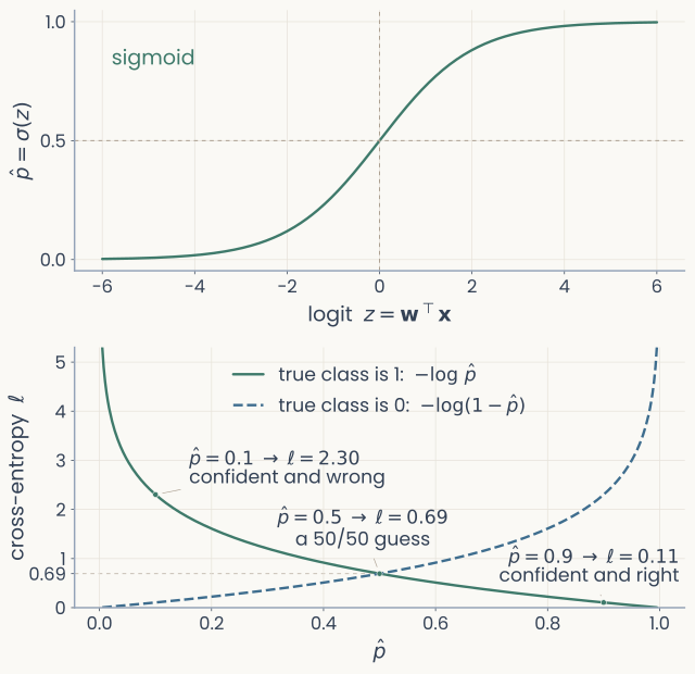
Two stacked panels. Top: the sigmoid curve, probability p-hat rising from 0 to 1 as the logit z goes from negative to positive, crossing 0.5 at z equals 0. Bottom: cross-entropy against p-hat; for a true class of 1 the loss falls from above 5 to 0 as p-hat goes to 1, and for a true class of 0 it rises the other way
Open full-size figure

Return to contents

Slide 28

Minute paper

Submit on Canvas → Minute papers → Minute Paper 9 (access code read out in class).

Write three brief points in your own words:

In the model neuron, what does a weight $w_i$ stand for in a real neuron, and what does a negative weight mean?
Something you do not yet understand, or a question still open
Another idea you found interesting, and why it matters for brains, behavior or AI

Credit for a thoughtful attempt, not for being correct.

Return to contents

Learning the weights: from neurons to gradient descent

Learning the weights: from neurons to gradient descent

You have been using model neurons all along

What a real neuron does

At a synapse: a spike becomes a current

From a neuron to a model neuron

Building the neuron: inputs, weights and sum

The weighted sum is a dot product

A neuron's weights set a decision boundary

One weight vector, two readings

A neuron is a feature detector: template matching

Building the neuron: activation and output

Transfer functions: the nonlinearity gg

From weights set by hand to weights learned

A network maps inputs to outputs

Where does the target come from?

How can a readout learn its weights from labeled examples?

The first learning neuron: the perceptron

Which way is downhill? From derivative to gradient

The delta rule (Widrow–Hoff): step down a smooth error

Try it: perceptron and delta rule, one example at a time

Logistic regression: a probability, then its error

Further reading for the research trail

Minute paper

Transfer functions: the nonlinearity $g$